약한 탄성 단층을 적용한 유한요소 모형을 이용한 지진 변형과 지진 후 변형에 대한 수치모사 연구

초록
지진에 의해 발생하는 지각 변형을 관측하고 그것을 지구동역학적으로 수치모사하면 지구 내부의 기계적 물성을 추정할 수 있다. 지진이 발생하면 지진 변형(coseismic deformation)과 지진 후 변형(postseismic deformation)이 발생하는데, 이를 연속체 역학으로 모사하기 위해 다수의 연구에서 유한요소법을 도입했다. 단층 미끄러짐은 불연속면에서 발생하는 현상으로 유한요소법으로 모사하기 어렵다. 본 연구에서는 낮은 전단 탄성계수를 가진 얇은 너비의 연속체의 형태로 단층을 근사한 수치모형을 개발하고, 기존 준 해석적, 측지학적 연구와 비교하였다. 점탄성 이완에 의한 지진 후 변형을 모사하기 위해 점탄성 하부지각과 맨틀 위에 탄성 상부지각과 단층을 배치하고 미끄러짐을 부가했다. 단층의 전단 탄성계수를 상부지각의 1/100 이하로, 단층 너비를 100 m로 설정하면, 지진 변형, 지진 후 변형이 준 해석적 모형 대비 ~20%의 차이를 보인다는 것을 확인했다. 지진 발생 후 상반과 하반이 단층 방향으로 끌려오며, 모형의 조건에 따라 그 속도가 0.01 cm/year 과 1 cm/year사이이다. 수십 년이 지나면 상반의 변형 방향이 바뀌고 결국 멈추게 되는데, 이는 단층의 재잠김 및 지진 간 변형(interseismic deformation)이다. 개발된 모형은 지진 사이클의 각 단계(지진 변형, 지진 후 변형, 지진 간 변형)를 모두 재현했다. 또한 하부지각과 맨틀의 점탄성 물성이 지진 후 변형을 일관되게 결정함을 제시했다. 긴 맥스웰 이완 시간이 정의되면 지진 후 변형 속도가 더 느리다. 예를 들어, 이완 시간이 1년과 50년일 때 상반의 지진 후 변형 속도가 각각 ~1 cm/year와 ~0.06 cm/year이다. 이 연구에서 개발한 모형이 보이는 지진 변형 및 지진 후 변형 양상과 하부 물성 사이의 강한 연관성은 약한 탄성체 단층을 맨틀과 하부지각의 강도 추정 연구에 도입할 수 있음을 의미한다.
Abstract
Mechanical strength of the Earth’s interior can be estimated using geodynamic modelling of crustal deformation induced by earthquake. Coseismic and postseismic deformation occur in upper and lower plates after seismic slip along faults. Various studies applied Finite Element Method (FEM) to simulate this deformation, in the framework of continuum mechanics. Seismic slip is difficult to be modelled by FEM due to its nature of discontinuous interface. In the present study, we developed a numerical model containing an elastic fault as a form of continuum with low shear modulus and narrow width. We compared our results with the previous quasi-analytical and geodetical studies on coseismic and postseismic deformation. We assigned a fault and its seismic slip in elastic upper crust overlying viscoelastic lower crust and mantle to simulate postseismic deformation controlled by viscoelastic relaxation. We found that our models showed ~20% difference in coseismic and postseismc deformation compared to previous quasi-analytical solution, when shear modulus of fault is ~0.01 of that of upper crust and fault width is ~100 m. The both of upper and lower plates moved toward the fault with 0.01 cm/year to 1 cm/year velocity, which is consistent with previous geodetic studies. After decades, the upper plate moved away from the fault and eventually stopped, which refers to fault re-locking and intereseismic deformation. Our model reproduced seismic cycle successfully, i.e., coseismic deformation, postseismic deformation, and interseismic deformation. Furthermore, our model showed that viscoelastic property of lower crust and mantle consistently determines postseismic deformation pattern. When Maxwell relaxation times are 1 year and 50 years, the scales of postseismic deformation are ~1 cm/year and 0.01 cm/year, respectively. This strong correlation between mechanical properties of Earth’s interiors and postseismic deformation indicates that our method of weak elastic thin fault can be adopted to estimate the strength of mantle and lower crust.
Keywords:
megathrust earthquake, coseismic deformation, postseismic deformation, finite element method, viscoelasticity키워드:
메가스러스트 지진, 지진 변형, 지진 후 변형, 유한요소법, 점탄성1. 서 론
판구조론상 수렴형 판 경계인 섭입대에서는 강한 지진 활동인 메가스러스트 지진(megathrust earthquake)이 발생한다(Suzuki et al., 2011; Lay et al., 2012). 큰 지진동(Gregor et al., 2012)과 지진해일(McCloskey et al., 2008)을 유발하는 메가스러스트 지진의 사이클을 정량적으로 이해하는 것은 효과적인 지진 재난 방재에 필수적이다. 기존의 지질학적, 지구물리학적, 측지학적 연구를 통해 지진 사이클을 크게, 단층 미끄러짐(coseismic slip), 지진 후 변형(postseismic deformation), 지진 간 변형(interseismic deformation)으로 구분했다(Wang et al., 2012; Hetland and Hager, 2005). 최근 지진 사이클을 이해하는데 자주 적용하는 방식은 지표 변위에 대한 시계열 측정과 그 측정값을 구속할 수 있는 수치모사 사이의 조합 연구다(예, Hu et al., 2004; Lundgren et al., 2009). 측지 기술의 발전으로 지진 사이클 전체를 아우르면서 지표 변위를 높은 정밀도로 측정할 수 있게 되었다. 레이더 간섭기법이나 상시 GPS (continuous Global Positioning System)가 고체 지구 연구에 적극적으로 도입되면서 순간적으로 수 cm에서 수 m (Feng and Jónsson, 2012; Song and Lee, 2019)의 큰 지표 변위를 일으키는 지진 변형 뿐만 아니라 상대적으로 긴 시간 동안(수십 년 단위; Bedford et al., 2013)의 연속적인 변위인 지진 후 변형 역시 관측할 수 있게 되었다.
지진 후 변형을 조절하는 물리 현상으로 지진 후 미끄러짐(afterslip; Hsu et al., 2006), 다공질탄성 반발(poroelastic rebound; Hu et al., 2004), 점탄성 완화(viscoelastic relaxation; Wahr and Wyss, 1980; Reilinger, 1986; Dalla Via et al., 2005) 등이 제시되고 있다. 지진 후 미끄러짐은 섭입대 단층면 아스페리티(asperity)의 복잡한 마찰 거동(Marone et al., 1991), 다공질 탄성 반발은 지진에 의해 유도되는 다공질 내 유체 흐름(Peltzer et al., 1998), 점탄성 완화는 암석권과 상부맨틀의 점탄성 거동(Wang et al., 2012)에 의존한다. 지진 후 변형 관측치를 목적하는 물리 현상의 틀에서 구속한다면 그 물리 현상을 조절하는 물성을 추정할 수 있을 것이다. 각 현상은 진앙으로부터의 거리나 지진이 발생한 후 경과 시간에 따라 지진 후 변형에 미치는 영향도가 상이하다. 지진 후 미끄러짐이나 다공질 탄성 반발은 진앙으로부터 근거리 영역(Gonzalez-Ortega et al., 2014; Tian et al., 2020)에서 지진 발생 수개월 내에(Jónsson et al., 2003; Chlieh et al., 2007), 점탄성 완화는 원거리(수백 km 단위; Freed et al., 2006; Shao et al., 2016) 영역에서 지진 발생 이후 수십 년 단위(Khazaradze et al., 2002; Ergintav et al., 2009)의 지진 후 변형을 설명할 수 있는 것으로 알려져 있다. 예를 들어, 2011년 3월 11일 규모 9.0의 동일본 대지진이 발생한 후 일본 해구에서 ~1,000 km 이상 떨어져있는 한반도가 해구 방향으로 지진 후 ~160일간 약 1-5 cm 이동한 것을 GPS 연구를 통해서 관측했다(Baek et al., 2012). 2004년 12월 26일에 규모 9.2의 수마트라 대지진이 발생하고 해구로부터 대륙방향으로 800-1,000 km 지점에 위치하는 태국과 말레이반도에서도 ~5년간 ~40 cm의 해구 방향 이동이 관측되었다(Wiseman et al., 2015).
암석권의 점탄성 완화 성질에 바탕을 둔 수치모형을 이용해 메가스러스트 지진 후 변형에 관한 측지학적 관측치를 구속한다면, 진앙 근처인 섭입대를 넘어 후열도 분지와 대륙의 기계적 강도 구조를 추정할 수 있을 것이다. 섭입판의 상판인 대륙판은 표면에서부터 상부지각, 하부지각, 상부맨틀로 순서로 구성되어 있다(Burov, 2011). 섭입대에서 지진이 발생하면 지진 변위에 대해 상부지각은 탄성 반응하며 온도와 압력이 높은 환경에 놓여있는 하부지각과 상부맨틀은 점탄성(viscoelastic) 반응을 보인다(Freed and Lin, 2001). 갑작스러운 지진 변형이 점탄성체인 하부지각과 상부맨틀에 가해지면 변형은 탄성에너지로 저장되었다가, 시간이 지남에 따라 점성 변형에 의해 소산한다. 소산에 따른 지진 후 변형의 진화 양상은 하부지각과 상부맨틀의 유변학적 점탄성 물성(예, 점성도 등)의해 결정되며, 이 점탄성은 온도(Karato et al., 2001) 및 맨틀 부분용융(Gerya and Meilick, 2011)에 의해 조절되므로 지구 심부의 열적/기계적 성질을 추론하는데 있어 지진 후 변형량 분석은 중요한 연구이다.
지구동역학에서는 메가스러스트 지진 변형과 점탄성 완화를 모사하기 위해 다양한 기법을 도입해왔다. 가장 지배적으로 적용된 기법 중 하나는 유한요소법(finite element method)으로 매질이 연속체라고 가정한다(So and Capitanio, 2017). 하지만, 단층면과 단층이 없는 부분은 본질적으로 불연속면과 연속체라는 차이점을 가지고 있다. 연속체 역학의 틀 내에서 불연속면인 단층과 그 단층의 미끄러짐을 모사하기 위해 다양한 기술이 이용되었다. 지진 후 변형은 연속체 내의 변형이므로 유한요소법으로 계산하기에 용이하지만 단층의 지진 미끄러짐은 서로 분리된 두 면이 미끄러지는 현상으로 유한요소 계산이 본질적으로 어렵다. 이러한 약점을 극복하기 위해, 절점분할법(Split node method; Melosh and Raefsky, 1981)과 영역분해법(domain decomposition approach; Aagaard et al., 2013) 등이 도입되었다. 절점분할법에서는 단층의 미끄러짐을 모사하기 위해 단층면을 기준으로 두 쌍의 절점군을 만들고 이중짝힘(double couple source)을 경계조건으로 설정하는 방식이다. 영역분해법은 단층면을 마찰경계로 가정하고 수직항력과 전단응력의 마찰 관계를 제3의 구속조건으로 도입하여 단층 미끄러짐을 모사한다. 두 기법은 성공적으로 지진 미끄러짐과 그에 따른 지진 후 변형을 모사했다. 그러나, 기존에 쓰이던 수많은 상용 유한요소 코드에 바로 적용할 수 없다는 점, 적용하더라도 코드의 구조 전체를 재구성해야만 하는 단점이 있어 제한적으로만 사용되어 왔다. 이 한계를 극복하기 위해서 So and Capitanio (2020)은 일반적인 상용 유한요소 코드인 ABAQUS에 일부 요소를 von-Mises 항복 강도 조건을 가진 소성(plastic) 단층으로 정의하여 지진 미끄러짐을 모사했으며, 결과적으로 단층면에서의 미끄러짐, 지진 수준의 미끄러짐 속도, 단층 간의 상호작용을 모두 성공적으로 모사했다. 그러나 응력과 변형량의 관계를 정의하는 강성행렬을 프로그래밍을 통해 수동 수정해야 하므로 단층을 유한요소 소프트웨어에 직관적으로 도입할 수 없었다.
상용 유한요소 소프트웨어인 콤솔 멀티피직스(COMSOL Multiphysics®; 이하, 콤솔)는 편리한 GUI (Graphic User Interface)를 기반으로 모사하고자 하는 구조체의 형태, 물성, 지배방정식, 요소의 크기 및 형상 함수의 차수 등을 자유롭게 선택할 수 있다는 장점(Lee and So, 2019; Jo and So, 2020)이 있어 우리나라를 포함해 전 세계적으로 널리 쓰이고 있다(Rodríguez-González et al., 2014; Ding and Lin, 2016). 콤솔은 다수의 지배방정식이 결합된 선형계를 조립할 수 있고, 지배방정식 간의 복잡한 결합도를 고려하여 선형계를 역산하는 병렬화된 해석기(solver)의 종류를 다양하게 선택할 수 있다. 본 연구에서는 콤솔 내에서 단층의 지진 미끄러짐과 그에 따른 지진 후 변형을 용이하게 모사하는 방법을 개발하고 기존 연구와 비교하고자 한다. 이 방법에서 도입한 단층 미끄러짐 방식에서는 두 단층면을 일정한 거리로 분리하고 그 사이에 탄성계수가 주변 지각에 비해 상대적으로 낮은 탄성체를 배치하여 빈 공간을 채운 후 그 공간을 둘러싼 두 면에서 반대 방향 미끄러짐을 가한다. 이 방식을 통해 유한요소 수치해석 소프트웨어인 콤솔에 단층을 도입하면서도 연속체 가정을 위배하지 않았다. 뿐만 아니라 So and Capitanio (2020)의 소성(plastic) 단층과 같은 복잡한 기법을 사용하지 않았다. Goodman et al. (1968)에서 본 연구와 유사하게 단층 사이에 두께가 0이고 매우 작은 탄성 계수를 가진 작은 요소를 도입하여 단층을 모사하려 시도했다. 그러나 주변부에 비해 작은 탄성 계수가 존재하여 기계적 강도 대비가 커지면 큰 계산량이 필요하여 광범위하게 시험되지 못했다. 뿐만 아니라 점탄성체가 포함된 계산 역시 시험하지 못했다. 이상적으로는 탄성계수가 작을수록 단층의 너비가 작을수록 실제 단층과 유사할 것으로 기대되지만 너무 작은 탄성계수와 너무 작은 단층 내 요소의 크기는 유한요소법의 부정확성을 유발하므로, 적절한 탄성 계수와 단층 너비를 탐색하는 최적화 과정은 이 기법에 있어 필수적이다. 이 연구에서는 탄성 계수와 단층면 사이의 거리를 변수로 설정하여 지진 변형과 지진 후 변형을 콤솔로 모사하고 콤솔의 지진 사이클 연구에 관한 타당성을 평가했다.
2. 연구 방법
2.1 지배방정식
본 연구에서는 3차원 지진 변형과 점탄성 지진 후 변형을 수치모사하기 위해 준정적(quasi-static) 운동량 보존 방정식을 지배방정식으로 도입하였다:
| (1) |
이 식에서 σij는 코시 응력 텐서(Cauchy’s stress tensor)이고, xj는 공간 좌표를 나타낸다. 본 연구에서는 지진 변형이 지진 후 변형에 미치는 효과만을 계산하고 지각 평형에 의한 효과는 무시하기 위해서 중력을 고려하지 않았다(Barbot and Fialko, 2010). 이 때, 응력 σij는 다시 편차 응력 텐서(deviatoric stress tensor) 와 등방응력(mean normal stress) σm으로 다음과 같이 분해된다:
| (2) |
δij는 크로네커델타(Kronecker delta)다. 본 연구에서 도입한 물성은 탄성과 점탄성이다. σij와 변위 ui사이의 관계를 조성 방정식으로 규정한다. 탄성이 정의된 영역은 다음과 같은 선형 탄성 조성 방정식을 따라 변형률(strain)과 응력의 관계가 결정된다:
| (3) |
εij, ui, G, K 는 각각 변형률 텐서, i 방향 변위, 전단 탄성 계수와 체적 탄성 계수를 의미한다. 변형률 텐서는 체적 변형률 텐서(volumetric strain-rate tensor) εvolδij와 편향 변형률 텐서 eij로 분해된다:
| (4) |
점탄성이 정의된 영역에서는 편향 변형률만이 다음과 같이 맥스웰(Maxwell) 점탄성 조성 방정식을 따르는 것으로 가정한다:
| (5) |
는 각각 편향 변형률 속도 텐서(deviatoric strain-rate tensor), 탄성 편향 변형률 속도 텐서(elastic deviatoric strain-rate tensor)와 점성 편향 변형률 속도 텐서(viscous deviatoric strain-rate tensor)이다. D/Dt와 η는 전미분과 점성도를 의미한다. 상기한 조성 방정식과 유한요소법을 이용해 선형계를 구성하고 이를 해석하여 각 요소의 절점에서 ui를 구한다.
2.2 수치모형의 구성
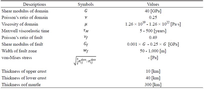
콤솔을 지진 변형 및 지진 후 변형 모사에 이용 가능한지 평가하기 위해, Segall (2010)의 해석 모형(이하, 해석 모형)과 비교하여 벤치마킹하였다. 해석 모형에서는 맥스웰 점탄성 반무한 공간(viscoelastic half-space) 위에 놓여있는 순수한 탄성 층에 포함된 단층의 미끄러짐과 그 이후의 지진 후 변형을 준 해석적 방법으로 풀이했다. 우리는 이 현상을 콤솔로 재현하기 위해 3차원 수치모형을 제작하였다(그림 1). 수치모형은 벤치마킹 대상인 해석 모형과 동일하게 상부지각, 하부지각, 맨틀로 구성되어 있으며, 각 층의 두께는 10 km, 40 km, 300 km로 설정했다. 상부지각은 탄성이며, 하부지각은 점탄성 물질로 정의했다. 상부지각 변형은 탄성판의 굽힘 등으로 일차적으로 설명된다(Bevis et al., 2004). 그에 비해, 지표에서 관측되는 시간 의존성 작은 변형(예, 지진 후 변형)은 하부지각이 점탄성이기 때문에 발생하는 것으로 알려져 있다(Pollitz et al., 2011). 맥스웰 점탄성 반무한 공간을 재현하기 위해서 상부지각에 비해 매우 깊은 점탄성 맨틀 공간을 설정했다. 상부지각에 전단 탄성 계수 G와 v포아송비 (표 1)를 설정하며, 하부지각과 맨틀에는 동적 점성도 η를 추가로 설정하였다. 따라서 맥스웰 이완 시간(Maxwell relaxation time) τM은 0.5·/η/G 이다.

a) Three dimensional model setup of coseismic and postseismic deformation. Our model is composed of three layers, i.e., elastic upper crust (green region), viscoelastic lower crust (blue region), and viscoelastic mantle (brown region). Yellow region indicates a fault. The fault is located at 140 km distance from an edge. The fault is approximated as a continuum elastic material with lower shear modulus Gf and thin width wf. We adopted 0.7 m and 0.3 m slip along the upper and lower planes of fault (see arrows in the inset of Fig. 1a). b) Mesh structure of the domain. We defined a small mesh around the fault, and enlarged the mesh near the edge (up to 50 km). We showed a zoomed-up view of mesh structure (see the inset of Fig.1b). The boundary condition of side walls and bottom is free-slip. The top is defined as free surface.

Description and values of variables.
탄성 상부지각에는 30도 경사를 가진 단층면을 정의했다(그림 1a). 단층을 모사하기 wf위해 (50-1,000 m)만큼 떨어진 두 단층면을 정의하고 그 사이에 주변 상부지각에 비해 매우 낮은 전단 탄성 계수 Gf(0.001 × G - 0.25 × G)를 가진 순수한 탄성 물질을 채웠다(그림 1a의 노란색 부분). 두 단층면에 미끄러짐 1m의 70%는 상반에, 30%는 하반에 적용했다(Pollitz et al., 2011). 최상부에는 자유경계면(free surface) 조건을, 그 외 모든 면에는 미끄럼 경계 조건(free slip)을 부가했다. 경계조건이 상부 변형에 미치는 효과를 최소화하기 위해 주향 방향으로 단층 규모(~10 km 수준)에 비해 30배 이상 긴 공간을 설정했다. 넓은 범위의 wf와 Gf값을 도입하여 콤솔이 지진 변형과 지진 후 변형을 기존 준 해석적 결과와 유사한 경향성을 가지고 재현하는지 확인하였다. 또한, 벤치마킹 결과를 바탕으로 지진이 발생한 후 이어지는 지진 후 변형이 하부지각의 점성도에 의존하는 간단한 수치모형 결과를 제공하고자 한다. 수치모사 공간은 4개의 절점으로 이뤄진 사면체 선형 요소로 이산화 했으며, 단층 주변 요소는 모형에 따라 0.5 km에서 1 km 길이 수준이며, 경계로 갈수록 요소의 크기가 커져 50 km이르도록 했다(그림 1b). 본 연구에서 구성한 선형계의 자유도(degree of freedom)는 100만에서 200만 사이이며, MUMPS (Multifrontal Massively Parallel sparse direct Solver; Amestoyet al., 2000) 해석기를 이용하여 각 절점에서의 변위를 구했다. 시간 단계(time-step)는 τM의 1/10 이하로 설정하여 점탄성 거동을 효율적으로 추적했다.
3. 결 과
해석 모형에서는 맥스웰 점탄성 반무한 공간 위에 놓여있는 탄성 상부지각과 그에 포함된 30도 경사를 가진 역단층의 미끄러짐에 의한 지진 변형과 지진 후 변형을 준 해석적으로 계산했다. 본 연구에서는, 콤솔로 제작한 3차원 유한요소 모형을 바탕으로 계산한 지진 변형과 지진 후 변형을 해석 모형의 결과에 벤치마킹하였다. 준 해석적 풀이와 달리 유한요소에서는 실제 단층면은 존재할 수 없으므로 본 연구에서는 낮은 탄성 계수를 가진 충진물을 단층으로 가정한 모형이 지진 변형과 지진 후 변형을 효과적으로 모사할 수 있는지 시험하였다.
3.1 참조모형
wf와 Gf에 각각 100 m와 0.01 × G를 모형에 도입한 후 참조모형(reference model)을 제작했다(그림 2). wf = 100 m는 단층의 길이(~20 km)에 비해 0.5%에 해당하는 길이이며, Gf는 주변의 온전한 상부지각의 전단 탄성 계수의 1%에 불과하다. 다수의 지구동역학 모형에서 단층, 약대, 전단대 등의 강도를 주변의 1/100 이하로 설정하는 것에 비춰보면 타당한 것으로 판단된다(Toth and Gurnis, 1998). 하부지각과 맨틀의 점성도 η = 1.26 × 10²⁰ Pa·s로, 모형의 전단 탄성 계수 G = 40 GPa로 설정하였기 때문에, 맥스웰 점탄성 이완 시간 τM은 약 50년이다. 계산은 시간이 τM이 될 때까지 수행하였다. 단층의 미끄러짐은 초기 조건으로 주어지는 것이므로 그에 따른 변형은 계산 수행 시간이 길어질수록 참값과의 오차가 커지게 될 것이다. 또한, 측지학으로 측정할 수 있는 지진 후 변형은 수십년 단위이므로 τM까지 본 연구에서 도출한 결과와 해석 모형의 결과가 유사하다면 콤솔을 실제 지구의 지진 변형과 지진 후 변형 연구에 도입할 수 있을 것으로 예상된다. 지진 후 변형은 지진 발생 후에도 100년 이상 지속될 수 있다고 알려져 있다(Vergnolle et al., 2003).

a) Three dimensional domain deformed by coseismic deformation. We exaggerated the deformation by 10000 and 5000 to vertical and horizontal displacements, respectively. Upper and lower plates moved upward and downward by 0.4 m and 0.2 m, respectively. b) Vertical (color) and horizontal (arrows) displacements of top surface. The upper plate showed leftward movement toward the fault (see black solid line). The amount of displacement decreased as the distance from fault increased. A localized vertical suppression is observed near the fault (see black dotted contour). c) The von-Mises stress (color) and displacement vectors (arrows) on a cross section along the red dotted line in Fig. 2b. The stress level around the fault is 1 to 10 MPa. On the other hand, the stress level is 0.01 MPa near the edges.
그림 2a에 계산 영역에 발생한 지진 변형을 3차원으로 도시하였다. 색은 수직 변위를 의미한다. 가시성을 위해 수직 방향으로 10,000배 수평 방향으로 5,000배 과장했다. 단층 근방에서는 상반과 하반이 각각 0.4 m, 0.2 m 변형한 것을 확인할 수 있다. 그림 2b는 모형의 최상부의 변형을 도시했다. 화살표는 수평 방향 지진 변위를, 색은 수직 방향 지진 변위를 의미한다. 빨간색과 파란색은 각각 상승과 하강을 의미한다. 단층의 상반과 하반이 각각 왼쪽과 오른쪽으로 이동하는 것을 확인했으며 단층 주변부에 압축력이 가해짐을 파악할 수 있다. 흥미로운 점은 상반 부분에 그림 2b의 검은색 점선 내부) 국지적인 0.1 m의 침강이 관찰되며, 이는 1700년 캐스캐디아 메가스러스트 지진 직후에 생긴 상반의 침강 흔적(Plafker, 1972; Leonard et al., 2004)과 유사하다. 경계조건 효과를 최대한 감소시키기 위해 모형의 중심부의 단면에서 지진 변위의 상부지각과 하부지각 내 분포를 확인할 수 있다. 그림 2c는 모형의 중심을 기준으로 자른 단면도이며(그림 2b의 빨간색 점선) 변위량에 따라 계산 영역을 변형하여 도시했다. 화살표는 변위, 색은 von-Mises 편차 응력을 의미한다. 단층 주변부에 1-10 MPa가량의 큰 응력이 존재한다. 이는 기존 지진 변형 수치모사 연구 결과와 유사한 값이다(예, Zhu and Zhang, 2013).
그림 3a-3d는 각각 지진 발생 후 0.4 × τM, 0.6 × τM, 0.8 × τM, 1.0 × τM의 시간이 경과했을 때 모형 최상부의 수직 방향 지진 후 변형량과 속도를 보여준다. 모든 시점에서 상반 부분이 단층 방향으로 끌려오는 모습을 보여주며, 이러한 형태의 지진 후 변형은 지구에서 전형적이며 해구의 메가스러스트 지진이나(Baek et al., 2012; Wiseman et al., 2015) 2008년 규모 7.9의 쓰촨 판내부지진(Jiang et al., 2017)에서도 측지학적으로 관측되었다. 모형 중심부의 단면도를 통해 하부지각의 변형을 관찰하면, 하반 부분과 상반 부분 모두 단층 방향으로 끌려가는 것을 확인할 수 있다(그림 1c). 그 속도가 0.1 cm/year에 이르며 이는 실제 GPS로 관측되는 값과도 차수가 동일하다(Vergnolle et al., 2003). 하반 부분의 지진 후 변형 역시 단층 방향으로 발생하는데 이는 2004년 수마트라 대지진(Reddy et al., 2010) 이후, 남인도 지역이나 2011년 동일본 대지진(Baek et al., 2012) 이후 한반도의 수평 변형 방향과도 유사하다.

The vertical displacement and velocity vectors of top surface at time of a) 0.4 × τM, b) 0.6 × τM, c) 0.8 × τM, and d) 1.0 × τM after coseismic slip. The fault-ward aseismic slip velocity is consistently observed in all time steps. The magnitude of velocity decreased with time. At time = 0.4 × τM and 1.0 × τM, the velocities of upper plate are 0.05 cm/year and 0.01 cm/year, respectively.
그림 4a-4d는 0.4 × τM, 0.6 × τM, 0.8 × τM, 1.0 × τM 시점에서 모형의 가운데 단면에서의 지진 후 변형 속도와 응력을 보여준다. 0.4 × τM 시점(그림 4a)와 1.0 × τM 시점(그림 4d)를 비교하면 지진 후 변형 속도가 현저히 감소한 것을 확인할 수 있다(화살표의 길이 비교). 색깔은 von-Mises 응력을 의미하는데, 단층 근처의 응력 수준이 시간이 지남에 따라서 감소한다. 즉, 지진에 의한 탄성 변형에 의한 응력이 시간에 따라 점탄성 이완하는 것을 지시한다. 더 자세히 응력 이완을 확인하기 위해서 그림 4a의 흰색과 검은 점선을 따라 응력 프로파일의 시계열 변화를 그림 5a와 5b에 각각 도시했다. 두 프로파일 모두 1.0 × τM 기간 동안 약 2,500 Pa에서 37,000 Pa 사이 정도의 점탄성 이완을 보이며(회색 화살표 부분 참조), τM이 50년임을 고려하면 평균 ~62 Pa/year에서 ~925 Pa/year 사이의 응력 변화 속도를 보인다. 이 값은 샌 안드레아스 단층에서 계산된 응력 부하 속도(50 Pa/year - 150 Pa/year; Parsons, 2002)와 차수가 일치한다.

Distribution of von-Mises stress and velocity vector on the cross section along the red dotted lines in Fig. 3a, at time of a) 0.4 × τM, b) 0.6 × τM, c) 0.8 × τM, and d) 1.0 × τM. The stress level near the fault relaxed with time (compare colors of Fig. 4a and 4d). The velocity is also reduced from ~0.05 cm/year to ~0.01 cm/year from time = 0.4 × τM to time = 1.0 × τM.

von-Mises Stress profiles along a) white and b) black dotted lines (see Fig. 4a), which starts from the points of lower and upper plates, respectively. The colors of indicate the time steps. In both figures, we observed apparent stress relaxation with time. For instance, at the depth = 8 km (see gray arrows in Fig. 5a), the amount of stress relaxation between time = 0.2 × τM to time = 1.0 × τM is 37000 Pa, which means that stress unloading rate is ~925 Pa/year. At shallow depth around 10 km, the unloading rate of upper plate (350 Pa/year; see gray arrows in Fig. 5b) is smaller than that of lower plate.
3.2 지진 변형과 지진 후 변형 비교
넓은 범위의 wf와 Gf값을 유한요소 수치모형에 도입하고 그 계산 결과를 해석 모형과 비교함으로써 정확하고 효율적인 콤솔 유한요소 계산을 위한 최적화된 wf와 Gf값 탐색하고자 한다. 계산 후, 단층 주향의 수직 방향의 선을 따라서 표면의 시간이 0 (지진 변형)일 때와 1 × τM (지진 후 변형)의 수평 변위와 수직 변위를 추출했다.
그림 6는 wf를 50 m로 고정하고 Gf값을 0.25 × G, 0.1 × G, 0.01 × G, 0.001 × G 로 설정한 후 계산한 결과를 보여준다. 검은색 실선과 점선은 시간이 0일때와 1 × τM일때 해석 모형이 도출한 수평 변위다. Gf가 0.25 × G인 경우(그림 6a)는 단층의 탄성이 충분히 작지 않은 상태로 간주할 수 있다. 지진 변형과 지진 후 변형이 모두 비교 대상과 확연한 차이가 있음을 확인할 수 있다. 단층의 근방(약 20 km 이내)은 지진 변형과 지진 후 변형이 해석 모형결과와 매우 상이하다. 하반의 변형을 더 작게 예측하며 상반의 변형은 더 크게 예측한다. 예를 들어, 해석 모형에서는 단층에서 하반의 수평 변위를 0.3 m, 상반의 수평 변위를 -0.6 m를 도출하지만 우리의 계산 결과는 각각 0.1 m 와 -1.5 m (그림에는 표현되어 있지 않음)으로 그 차이가 크다. Gf가 0.1 × G인 모형(그림 6b)은 하반의 변위는 그림 6a의 경우에 비해 개선되었으나 여전히 상반의 변위를 크게 측정한다. Gf가 0.01 × G, 0.001 × G인 경우(그림 6c와 6d), 단층 주변의 수평 방향 지진 변형과 지진 후 변형이 모두 유사함을 확인하였다. 두 모형 모두 단층을 경계로 하반과 상반의 수평방향 움직임을 대략 0.2 m와 -0.6 m를 도출하여 해석 모형과 유사하다. 해석 모형은 단층에서 먼 상반에서 복잡한 변위를 보여준다. 상반의 15 km지점과 25 km 지점에서 각각 국지적 최댓값과 최솟값을 보여준다. Gf가 0.01 × G, 0.001 × G인 모형은 이 경향성을 동일하게 재현한다. 그러나, 전체적으로 상반에서의 수평 변형에 대해서 유한요소 모형이 준 해석 모형에 비해 강한 변위를 예측하는 것으로 판단된다. 또한, 하반의 변형은 유한요소 모형과 준 해석 모형이 거의 유사하게 예측한다. Gf = 0.01 × G와 Gf = 0.001 × G인 경우의 결과가 거의 동일한데, 이는 Gf = 0.01 × G이 계산의 효율성과 정확성을 모두 확보할 수 있는 단층 내 물질의 탄성 계수임을 지시한다. 그림 7은 값을 0.01 × G로 고정하고 wf값을 50, 100, 500, 1,000 m로 설정하고 계산한 수평 변위 분포다. 그림 7a-d의 네 모형 모두 단층 주변부의 수평 변위가 Segall (2010)과 거의 일치한다. 모든 모형이 단층으로부터 거리가 0인 지점에서 하반과 상반은 각각 0.3 m와 -0.6 m가량의 지진 변형과 지진 후 변형을 보이며 해석 모형이 도출한 값과도 일치한다. 또한 모든 모형이 해석 모형과 유사한 값의 하반 변형을 보인다. 상반의 변형은 값에는 차이가 있지만 국지적 최대값과 최솟값이 존재하는 위치가 수치 모형과 해석 모형이 일치한다.

Coseismic and postseismic horizontal displacements between our models (blue and red lines) and semi-analytical solution (black solid and dotted lines; Segall, 2010) with varying Gf and fixed wf = 50 m. Figs. 6a-6d show horizontal displacement along the central line over top surface for the cases of a) Gf = 0.25 × G, b) 0.1 × G, c) 0.01 × G, and d) 0.001 × G, respectively. When Gf = 0.25 × G, our model predicted far different results from the semi-analytical solutions.

Coseismic and postseismic horizontal displacements with varying wf and fixed Gf = 0.01 × G. We tested four cases with a) wf = 50 m, b) wf = 100 m, c) wf = 500 m, and d) wf = 1,000 m. All of cases result in similar pattern, which indicated that the pattern is not sensitive to values of wf when Gf is sufficiently small as 0.01 × G.
그림 8은 지진 변형 중 수직 변위를 보여준다. wf를 50 m로 고정하고 Gf값을 0.25 × G, 0.1 × G, 0.01 × G, 0.001 × G 변경하며 수직 변위를 계산하고 비교하였다. Gf값이 0.25 × G이면(그림 8a) 단층의 근방에서는 상반의 상승을 작게 예측하고 하반의 하강을 크게 추정하는 경향이 있다. 단층에서 멀리 떨어진(30 km 이상) 상반 부분의 변위는 정확히 일치하지는 않지만 경향성이 유사하다. Gf값이 0.01 × G와 0.001 × G이면 단층 주변과 먼 곳의 변위를 매우 유사하게 추정하며 Gf = 0.01 × G과 Gf = 0.001 × G (그림 8c와 8d)의 결과가 거의 동일하다. 그림 9는 Gf값을 0.01 × G로 고정하고 wf값을 50, 100, 500, 1,000 m 로 변경하며 구한 수직 변위이다. 수직 변위는 어떤 wf값을 도입하더라도 Gf값이 0.01 × G로 충분히 작아 준수한 결과를 보였다.

Coseismic and postseismic vertical displacements with varying Gf and fixed wf = 50 m. When Gf = 0.25 × G (Fig. 8a) and Gf = 0.1 × G (Fig. 8b), vertical displacement patterns are different with semi-analytical solution (black solid and dotted lines). Our model predicted smaller upward motion of upper plate compared to that of the analytical solution. On the other hand, the cases of Gf = 0.01 × G (Fig. 8c) and Gf = 0.001 × G (Fig. 8d) deduced similar results.

Coseismic and postseismic horizontal deformation with varying wf and fixed Gf = 0.01 × G. The cases of a) wf = 50 m, b) wf = 100 m, c) wf = 500 m, and d) wf = 1,000 m resulted in similar displacement patterns, as well as similar to semi-analytical solution.
3.3 최적화된 단층의 너비와 전단 탄성계수
해석 모형과 우리의 유한요소 모형 사이의 비교 결과를 정량화 하기 위해서 넓은 범위의 wf(5 m ≤ wf ≤ 1,000 m)와 Gf(G/2 ≤ Gf ≤ G/1024)값을 적용하여 110개의 유한요소 모형 계산을 수행했다. 지진 변형과 지진 후 변형의 해석 모형의 결과와의 차이를 RMSD (Root-Mean-Square Difference)로 표현했다(그림 10). 그림 10a는 지진 변형 중 수평 변위에 관한 결과이다. 대체로 RMSD는 wf가 작을수록 작아진다. wf가 5 m일때, Gf = G/2인 경우(주황색 선)와 Gf = G/1024인 경우(남색 선)의 경우 차이가 각각 ~0.23와 ~0.18이다. 같은 Gf인 경우 wf가 커진다고 RMSD가 크게 변하지 않는다. 다만, Gf = G/1024인 경우 wf가 커질수록 RMSD가 작아지는 것을 확인했다. 그에 비해 Gf = G/128(갈색 선)일 때는 wf가 변한다고해도 RMSD는 0.18 정도로 일정하다. 우리의 모형은 해석 모형에 비해 10%에서 20% 정도의 결과값 차이가 있지만, 해석 모형 역시 반무한 공간 가정을 썼음을 감안하면 해당 wf와 Gf값이 지진 변형을 위한 유한요소 계산에 사용될 수 있을 것으로 판단된다. 그림 10b에 시간이 τM인 시점에서 수평 방향의 지진 후 변형에 있어서 RMS 차이를 도시했다. Gf = G/2로 단층을 대신하는 퇴적 충진물의 강도가 충분히 강하면 RMSD가 ~0.4로 매우 크다. 대체로 지진 변형과 유사한 결과를 보여주며 Gf = G/128(갈색 선)일 때 wf값에 상관없이 RMSD가 ~0.14로 일정하다.

Root-Mean-Square Difference (RMSD) of horizontal/vertical and coseismic/postseismic deformation between our model and the semi-analytical solution with a wide range of wf and Gf. We showed RMSD of horizontal a) coseismic and b) postseismic deformation, and vertical c) coseismic and d) postseismic deformation with varying wf and Gf.
그림 10c는 수직 변위의 RMSD를 보여준다. wf가 일정하면 Gf가 작아질수록 RMSD가 더 작다는 점에서 수평 변위의 RMSD의 경향성이 비슷하다. 그러나, 일정한 Gf를 가질 때 wf가 커질수록 RMSD가 커진다. 대체로, wf = 100 m일때 국지적인 최소 RMSD를 보이며, 특히 Gf가 G/128이하면 RMSD가 ~0.11정도로 최저이다. 지진 후 변형의 수직 변위(그림 10d)의 경우 대체로 수평 변위에 비해 RMSD가 더 크다. Gf가 G/128 이하일 때 RMS가 ~0.22으로 최저값을 보인다. 그림 10a-10d를 종합하면 Gf가 G/128 이하이며 wf가 100 m일 때 지진 변형과 지진 후 변형의 수직/수평 변위의 RMSD가 0.22 미만이며, 이 Gf와 wf값이 유한요소를 이용한 단층 제작에 적합한 값으로 판단된다.
wf의 값이 작아질수록 더 작은 요소가 필요하기 때문에 더 높은 자유도(degree of freedom, DOF)를 가진 수치모형을 필요로 한다. 실제로 콤솔에서 제공하는 자동 격자 생성기를 이용하면 wf = 50 m일 때 약 1백만 DOF이며 wf가 커질수록 대체로 감소하여 wf = 1,000 m일 때는 85만이다(그림 11 빨간색 점선). 계산의 효율성을 확인하기 위해서 계산 코어의 개수를 8개로 고정하고 넓은 범위와 wf와 Gf를 도입한 다수의 모형에서 해석 시간을 측정하였다. 그 결과 wf가 커질수록 대체로 계산 시간이 감소하는 것을 확인할 수 있다. wf = 50 m인 경우와 wf = 100 m인 경우가 계산 시간에 가장 큰 차이를 보이며, wf = 100 m이면 Gf가 G/128과 Gf가 G/256일때 가장 짧은 계산 시간을 보인다. 우리는 그림 10과 11을 종합하여 wf = 100 m 과 Gf = G/128이 콤솔을 이용한 유한요소 단층 미끄러짐과 그에 따른 지진 변형과 지진 후 변형을 모사하기에 최적의 값이라고 결론 내렸다.

Wall time of finite element calculation with different values of wf and Gf. Red dotted line indicated the degree of freedom (DOF) with varying wf values. DOF and wall time are roughly decreased with increasing wf. We fixed number of cores and RAM at 8 (Intel Core i7 @ 3.4 GHz) and 16 Gb RAM, respectively.
3.4 맥스웰 점탄성 이완 시간과 지진 후 변형
앞서 특정한 wf와 Gf값을 적용하여 다양한 맥스웰 이완 시간(즉, 다양한 맨틀 점성도) τM을 대입하여 추가 수치모사를 수행했다. 우리는 wf = 100 m 와 Gf = G/128로 고정하고 τM을 5년에서 500년 사이로 설정한 수치모형을 제작했다. 그림 12에 이완 시간, 상반/하반, 단층으로부터 거리에 따른 수평 방향 변위의 시계열 변화를 도시했다. 모든 그림에서 시간이 0일때 갑작스러운 변위가 보이는데 이는 지진 변형이다. 그림 12a에는 단층으로부터 40 km 떨어진 하반의 한 점의 시간에 따른 수평 방향 지진 후 변형을 도시했다. 우리의 모형에서는 하반이 오른쪽으로 움직이므로 변형량을 양수로 표시했다. τM이 5년(파란색 선)이면 지진 발생 후 100년 간 0.15 cm/year의 속도로 단층 방향으로 끌려간다, τM이 500년(녹색 선)이면 0.007 cm/year의 속도를 보여준다. 그림 12b에는 단층으로부터 80 km 떨어진 하반의 한 점의 수평 방향 지진 후 변형이다. 거리가 멀어짐에 따라 지진 후 변형의 양도 감소한다. 예를 들어, τM이 5년(파란색 선)일 때 그림 12a에서는 100년 시점에 ~18 cm 이동했으나 그림 12b에서는 ~12 cm 이동하였다. 그림 12a와 12b를 종합하면 τM이 커짐에 따라 일관되게 지진 후 변형이 느려지는 것을 확인할 수 있다. 지진 후 변형의 속도가 시간이 지날수록 0에 가까워지는데 이는 지진 미끄러짐에 의한 탄성 에너지가 모두 소산했음을 의미한다.

Time series of horizontal postseismic displacement of lower (Figs. 12a and 12b) and upper (Figs. 12c and 12d) plates with different Maxwell viscoelastic relaxation time τM of lower crust and mantle when wf = 100 m and Gf = G/128. We extracted the displacements at each two points (40 km and 80 km away from the fault) in upper and lower plates. Lower plate (Figs. 12a and 12b) showed rightward postseismic motion. The larger τM is assigned, the quicker cessation of postseismic deformation is shown (compare blue and green lines). In upper plate, the leftward deformation after seismic slip is observed. However, the counter motion of upper plate (i.e., rightward motion) after a certain time values is found consistently with τM = 5, 50, and 100 years.
그림 12c와 12d는 단층으로부터 40 km와 80 km 떨어진 상반의 두 점에서의 수평 방향 지진 후 변형이다. 단층에서 가까울수록 더 큰 지진 후 변형이 있다는 점, τM이 길수록 더 느린 변형을 보여준다는 점 등이 하반의 변형 양상과 유사하다. 그러나, 변형의 방향이 바뀐다는 차이점이 있다. 이는 단층 재잠김(fault relocking)이 일어나는 것을 지시한다. 그림 12c의 파란색 선을 확인하면 지진 발생 후 30년간 단층 방향(즉, 왼쪽)으로 이동하지만, 그 이후는 다시 단층에서 멀어지다가(즉, 오른쪽), 지진 발생 후 200년이 지나면 결국 이동이 멈추게 된다. 이는 Hu et al. (2004)의 유한요소 수치모형에서 예측한 결과와 유사하다. Hu et al. (2004)은 맨틀의 점성도가 1 × 10²⁰ Pa·s일때 상판의 지진 후 변형 속도가 단층 방향에서 단층 반대 방향으로 지진 발생 후 35년 후에 전환되는 결과를 도출했다. 2004년 수마트라 지진의 상판에서 관측되는 지진 후 변형은 단층 방향, 1960년 칠레 지진과 1700년 캐스캐디아 지진에 의한 변형은 단층에서 멀어지는 방향이다(Wang et al., 2012). 우리의 모형이 τM에 따라서 일관된 지진 후 변형 경향성을 보인다는 것, 상판의 변형 방향이 특정 시점에 바뀐다는 점 등을 고려하면, 본 유한요소 모형은 지진 후 변형을 수치모사하여 맨틀과 하부지각의 물성을 파악하는데 유효하게 사용될 수 있을 것으로 판단된다.
4. 토의 및 결론
우리는 유한요소법을 이용해서 지진 발생에 의한 지진 변형과 지진 후 변형을 수치모사하고 그 효율성과 정확성을 파악하였다. 유한요소법의 기반이 되는 연속체 역학에 위배되는 단층을 도입하기 위해서 약한 탄성 물질을 채운 얇은 단층을 도입 및 시험하여 가장 적합한 단층의 물성과 너비를 탐색하였다. 우리는 단층의 탄성 물성과 너비가 결과에 민감하게 영향을 미치는 것을 확인했다. 광범위하게 변수 탐색을 하였으며 그 결과 단층의 전단 탄성 계수를 주변 상부지각의 ~1/100정도로, 단층 너비를 100 m로 설정하면 Segall (2010)의 해석 모형 결과와 가장 유사하다. 비교 대상이 수평 변위, 수직 변위, 지진 변형, 지진 후 변형인지에 따라 유사도는 다르지만 위에 제시한 값일 때 차이가 20% 이내로 가장 적합한 것으로 판단된다. 해석 모형 역시 반무한 공간 등의 다양한 가정을 사용한 것을 감안하면 본 연구의 유한요소 모형 대비 유사도는 타당한 것으로 보인다. 기존의 다수의 수치모사 연구 결과 및 측지학 연구 결과와 비교한 결과, 우리 모형이 보여주는 지진 후 변형의 경향성, 즉 i) 지진 발생 직후 상반과 하반이 모두 단층으로 끌려온다는 점, ii) 시간이 지나면 상반의 이동 방향이 단층에서 멀어지는 방향으로 바뀌면서 재잠김이 발생한다는 점, iii) 하부지각과 맨틀의 맥스웰 점탄성 이완 시간에 따라 지진 후 변형 속도가 일관성 있게 결정된다는 점, iv) 점탄성 이완에 따라 단층 주변부의 응력이 이완한다는 점 등이 기존 연구와 일맥상통함을 확인했다. 이는 우리 모형을 측지 관측 결과를 바탕으로 맨틀의 물성을 역산하는 연구에 도입할 수 있음을 의미한다.
본 연구에서는 지각과 맨틀의 기계적 물성을 지나치게 단순화한 경향이 있다. 측지 자료를 유한요소법으로 더 자세하게 구속하기 위해서는 실제 자연과 유사한 조건을 도입하고 시험해야한다. 표면에서 관측되는 지진 후 변형의 속도와 양에 큰 영향을 주는 맥스웰 점탄성 이완시간은 전단 탄성 계수와 점성도로 결정된다. 본 연구에서는 전단 탄성 계수를 모두 일정하게 설정했다. 향후 연구에서 Preliminary Reference Earth Model (PREM; Dziewonski & Anderson, 1981)등을 도입하면 더 상세한 탄성 구조를 제작할 수 있을 것으로 기대된다(Diao et al., 2013). 점성도 역시 지온 구배나 변형률 속도에 따라 크게 변화하므로 확산포행(diffusion creep)과 전위포행(dislocation creep)을 도입하면 상세한 점성도 구조를 적용할 수 있다(Peña et al., 2020). 향후, 섭입판의 기하학적 형태를 슬랩 1.0 (Slab 1.0; Hayes et al., 2012)등의 모형을 이용하면 탄성 섭입판이 지진 변형과 지진 후 변형에 미치는 영향을 상세히 모사할 수 있을 것이다. 우리 모형에는 지진 후 미끄러짐(afterslip)을 적용하지 않았다. 진앙에서 원거리 지역, 지진 후 수년 이후 지진 후 변형은 본 연구에서 다룬 점탄성 이완에 의존하는 것으로 알려져 있지만, 지진 사이클 전체를 아우르는 모형을 개발하기 위해서는 지진 후 미끄러짐 역시 고려해야할 것이다.
2011년 동일본 대지진 이후 한반도에도 지진 후 변형이 발생했다(Baek et al., 2012). 진앙에서 1,000 km이상의 원거리인데 지진 후 변형이 발생한 것을 고려하면 진앙과 한반도 사이에 존재하는 동해 하부 점성도에 대한 심도 있는 논의가 필요하다. 본 연구의 모형에 따르면, 점성도가 클수록 오랜 시간 동안 그리고 멀리까지 지진 후 변형이 작용한다. 하지만 본 연구에서는 그 경향성만을 파악했으며, 향후 우리 모형에 상세한 점성구조 및 탄성구조를 도입하면 동해 하부의 점성 구조를 파악할 수 있을 것으로 기대된다.
Acknowledgments
본 연구는 “행정안전부 방재안전분야 전문인력 양성”사업과 기상청 기상·지진 See-At 기술개발사업(KMI2018-02110), 2020년도 정부(교육부)의 재원으로 한국연구재단의 지원을 받아 수행된 신진연구지원 사업(NRF-2019R1C1C1010804)과 기초연구사업(No.2019R1A6A1A03033167)으로 수행되었습니다. 편집위원과 익명의 심사위원 2분께 감사의 말씀을 올립니다.
References
-
Aagaard, B.T., Knepley, M.G. and Williams, C.A., 2013, A domain decomposition approach to implementing fault slip in finite-element models of quasi-static and dynamic crustal deformation. Journal of Geophysical Research: Solid Earth, 118, 3059-3079.
[https://doi.org/10.1002/jgrb.50217]

-
Amestoy, P.R., Duff, I.S. and L'Excellent, J.-Y., 2000, Multifrontal parallel distributed symmetric and unsymmetric solvers. Computer Methods in Applied Mechanics and Engineering, 184, 501-520.
[https://doi.org/10.1016/S0045-7825(99)00242-X]
-
Baek, J., Shin, Y., Na, S., Shestakov, N.V., Park, P. and Cho, S., 2012, Coseismic and postseismic crustal deformations of the Korean Peninsula caused by the 2011 Mw 9.0 Tohoku earthquake, Japan, from global positioning system data. Terra Nova, 24, 295-300.
[https://doi.org/10.1111/j.1365-3121.2012.01062.x]
-
Barbot, S. and Fialko, Y., 2010, A unified continuum representation of post-seismic relaxation mechanisms: semi-analytic models of afterslip, poroelastic rebound and viscoelastic flow. Geophysical Journal International, 182, 1124-1140.
[https://doi.org/10.1111/j.1365-246X.2010.04678.x]
-
Bedford, J., Moreno, M., Li, S., Oncken, O., Baez, J.C., Bevis, M., Heidbach, O. and Lange, D., 2016, Separating rapid relocking, afterslip, and viscoelastic relaxation: An application of the postseismic straightening method to the Maule 2010 cGPS. Journal of Geophysical Research: Solid Earth, 121, 7618-7638.
[https://doi.org/10.1002/2016JB013093]
-
Bevis, M., Kendrick, E., Cser, A. and Smalley, R., 2004, Geodetic measurement of the local elastic response to the changing mass of water in Lago Laja, Chile. Physics of the Earth and Planetary Interiors, 141, 71-78.
[https://doi.org/10.1016/j.pepi.2003.05.001]
-
Burov, E.B., 2011, Rheology and strength of the lithosphere. Marine and Petroleum Geology, 28, 1402-1443.
[https://doi.org/10.1016/j.marpetgeo.2011.05.008]
-
Chlieh, M., Avouac, J., Hjorleifsdottir, V., Song, T.A., Ji, C., Sieh, K., Sladen, A., Hebert, H., Prawirodirdjo, L., Bock, Y. and Galetzka, J., 2007, Coseismic Slip and Afterslip of the Great Mw 9.15 Sumatra–Andaman Earthquake of 2004. Bulletin of the Seismological Society of America, 97, S152-S173.
[https://doi.org/10.1785/0120050631]
-
Dalla Via, G., Sabadini, R., De Natale, G. and Pingue, F., 2005, Lithospheric rheology in southern Italy inferred from postseismic viscoelastic relaxation following the 1980 Irpinia earthquake. Journal of Geophysical Research: Solid Earth, 110, B06311.
[https://doi.org/10.1029/2004JB003539]
-
Diao, F., Xiong, X., Wang, R., Zheng, Y., Walter, T.R., Weng, H. and Li, J., 2013, Overlapping post-seismic deformation processes: afterslip and viscoelastic relaxation following the 2011 Mw 9.0 Tohoku (Japan) earthquake. Geophysical Journal International, 196, 218-229.
[https://doi.org/10.1093/gji/ggt376]
-
Ding, M. and Lin, J., 2016, Deformation and faulting of subduction overriding plate caused by a subducted seamount. Geophysical Research Letters, 43, 8936-8944.
[https://doi.org/10.1002/2016GL069785]
-
Dziewonski, A.M. and Anderson, D.L., 1981, Preliminary reference Earth model. Physics of the Earth and Planetary Interiors, 25, 297-356.
[https://doi.org/10.1016/0031-9201(81)90046-7]
-
Ergintav, S., McClusky, S., Hearn, E., Reilinger, R., Cakmak, R., Herring, T., Ozener, H., Lenk, O. and Tari, E., 2009, Seven years of postseismic deformation following the 1999, M = 7.4 and M = 7.2, Izmit-Düzce, Turkey earthquake sequence. Journal of Geophysical Research: Solid Earth, 114, B07403.
[https://doi.org/10.1029/2008JB006021]
-
Feng, G. and Jónsson, S., 2012, Shortcomings of InSAR for studying megathrust earthquakes: The case of the Mw9.0 Tohoku-Oki earthquake. Geophysical Research Letters, 39, L10305.
[https://doi.org/10.1029/2012GL051628]
-
Freed, A.M., Bürgmann, R., Calais, E., Freymueller, J. and Hreinsdóttir, S., 2006, Implications of deformation following the 2002 Denali, Alaska, earthquake for postseismic relaxation processes and lithospheric rheology. Journal of Geophysical Research: Solid Earth, 111(B1).
[https://doi.org/10.1029/2005JB003894]
-
Freed, A.M. and Lin, J., 2001, Delayed triggering of the 1999 Hector Mine earthquake by viscoelastic stress transfer. Nature, 411, 180-183.
[https://doi.org/10.1038/35075548]
-
Gerya, T.V. and Meilick, F.I., 2011, Geodynamic regimes of subduction under an active margin: effects of rheological weakening by fluids and melts. Journal of Metamorphic Geology, 29, 7-31.
[https://doi.org/10.1111/j.1525-1314.2010.00904.x]
-
Gonzalez-Ortega, A., Fialko, Y., Sandwell, D., Alejandro Nava-Pichardo, F., Fletcher, J., Gonzalez-Garcia, J., Lipovsky, B., Floyd, M. and Funning, G., 2014, El Mayor-Cucapah (Mw 7.2) earthquake: Early near-field postseismic deformation from InSAR and GPS observations. Journal of Geophysical Research: Solid Earth, 119, 1482-1497.
[https://doi.org/10.1002/2013JB010193]
- Goodman, R., Taylor, R. and Brekke, T., 1968, A model for the mechanics of jointed rock. Journal of the Soil Mechanics and Foundations Division, 94, 637-659.
-
Gregor, N.J., Silva, W.J., Wong, I.G. and Youngs, R.R., 2002, Ground-Motion Attenuation Relationships for Cascadia Subduction Zone Megathrust Earthquakes Based on a Stochastic Finite-Fault Model. Bulletin of the Seismological Society of America, 92, 1923-1932.
[https://doi.org/10.1785/0120000260]
-
Hayes, G.P., Wald, D.J. and Johnson, R.L., 2012, Slab1.0: A three-dimensional model of global subduction zone geometries. Journal of Geophysical Research: Solid Earth, 117, B01302.
[https://doi.org/10.1029/2011JB008524]
-
Hetland, E.A. and Hager, B.H., 2005, Postseismic and interseismic displacements near a strike-slip fault: A two-dimensional theory for general linear viscoelastic rheologies. Journal of Geophysical Research: Solid Earth, 110, B10401.
[https://doi.org/10.1029/2005JB003689]
-
Hsu, Y., Simons, M., Avouac, J., Galetzka, J., Sieh, K., Chlieh, M., Natawidjaja, D., Prawirodirdjo, L. and Bock, Y., 2006, Frictional Afterslip Following the 2005 Nias-Simeulue Earthquake, Sumatra. Science, 312, 1921.
[https://doi.org/10.1126/science.1126960]
-
Hu, Y., Wang, K., He, J., Klotz, J. and Khazaradze, G., 2004, Three-dimensional viscoelastic finite element model for postseismic deformation of the great 1960 Chile earthquake. Journal of Geophysical Research: Solid Earth, 109, B12403.
[https://doi.org/10.1029/2004JB003163]
-
Jiang, Z., Yuan, L., Huang, D., Yang, Z. and Chen, W., 2017, Postseismic deformation associated with the 2008 Mw 7.9 Wenchuan earthquake, China: Constraining fault geometry and investigating a detailed spatial distribution of afterslip, Journal of Geodynamics, 112, 12-21.
[https://doi.org/10.1016/j.jog.2017.09.001]
- Jo, T. and So, B.D., 2020, Numerical Modeling of Shear Heating in 2D Elastoplastic Extensional Lithosphere using COMSOL Multiphysics®. Geophysics and Geophysical Exploration, 23, 1-12.
-
Jónsson, S., Segall, P., Pedersen, R. and Björnsson, G., 2003, Post-earthquake ground movements correlated to pore-pressure transients. Nature, 424, 179-183.
[https://doi.org/10.1038/nature01776]
-
Karato, S., Riedel, M.R. and Yuen, D.A., 2001, Rheological structure and deformation of subducted slabs in the mantle transition zone: implications for mantle circulation and deep earthquakes. Physics of the Earth and Planetary Interiors, 127, 83-108.
[https://doi.org/10.1016/S0031-9201(01)00223-0]
-
Khazaradze, G., Wang, K., Klotz, J., Hu, Y. and He, J., 2002, Prolonged post-seismic deformation of the 1960 great Chile earthquake and implications for mantle rheology. Geophysical Research Letters, 29, 7-1-7-4
[https://doi.org/10.1029/2002GL015986]
-
Lay, T., Kanamori, H., Ammon, C.J., Koper, K.D., Hutko, A.R., Ye, L., Yue, H. and Rushing, T.M., 2012, Depth-varying rupture properties of subduction zone megathrust faults. Journal of Geophysical Research: Solid Earth, 117, B04311.
[https://doi.org/10.1029/2011JB009133]
-
Lee, S.H. and So, B., 2019, Two dimensional finite element numerical model for slab detach- ment using Arbitrary Lagrangian Eulerian and remeshing. Journal of the Geological Society of Korea, 55, 663-682 (in Korean with English abstract).
[https://doi.org/10.14770/jgsk.2019.55.6.663]
-
Leonard, L.J., Hyndman, R.D. and Mazzotti, S., 2004, Coseismic subsidence in the 1700 great Cascadia earthquake: Coastal estimates versus elastic dislocation models. GSA Bulletin, 116, 655-670.
[https://doi.org/10.1130/B25369.1]
-
Lundgren, P., Hetland, E.A., Liu, Z. and Fielding, E.J., 2009, Southern San Andreas-San Jacinto fault system slip rates estimated from earthquake cycle models constrained by GPS and interferometric synthetic aperture radar observations. Journal of Geophysical Research: Solid Earth, 114, B02403.
[https://doi.org/10.1029/2008JB005996]
-
Marone, C.J., Scholtz, C.H. and Bilham, R., 1991, On the mechanics of earthquake afterslip. Journal of Geophysical Research: Solid Earth, 96, 8441-8452.
[https://doi.org/10.1029/91JB00275]
-
McCloskey, J., Antonioli, A., Piatanesi, A., Sieh, K., Steacy, S., Nalbant, S., Cocco, M., Giunchi, C., Huang, J. and Dunlop, P., 2008, Tsunami threat in the Indian Ocean from a future megathrust earthquake west of Sumatra. Earth and Planetary Science Letters, 265, 61-81.
[https://doi.org/10.1016/j.epsl.2007.09.034]
- Melosh, H.J. and Raefsky, A., 1981, A simple and efficient method for introducing faults into finite element computations. Bulletin of the Seismological Society of America, 71, 1391-1400.
-
Parsons, T., 2002, Post-1906 stress recovery of the San Andreas fault system calculated from three-dimensional finite element analysis. Journal of Geophysical Research: Solid Earth, 107, ESE 3-13.
[https://doi.org/10.1029/2001JB001051]
-
Peltzer, G., Rosen, P., Rogez, F. and Hudnut, K., 1998, Poroelastic rebound along the Landers 1992 earthquake surface rupture. Journal of Geophysical Research: Solid Earth, 103, 30131-30145.
[https://doi.org/10.1029/98JB02302]
-
Peña, C., Heidbach, O., Moreno, M., Bedford, J., Ziegler, M., Tassara, A. and Oncken, O., 2020, Impact of power-law rheology on the viscoelastic relaxation pattern and afterslip distribution following the 2010 Mw 8.8 Maule earthquake. Earth and Planetary Science Letters, 542, 116292.
[https://doi.org/10.1016/j.epsl.2020.116292]
-
Plafker, G., 1972, Alaskan earthquake of 1964 and Chilean earthquake of 1960: Implications for arc tectonics. Journal of Geophysical Research, 77, 901-925.
[https://doi.org/10.1029/JB077i005p00901]
-
Pollitz, F.F., Bürgmann, R. and Banerjee, P., 2011, Geodetic slip model of the 2011 M9.0 Tohoku earthquake. Geophysical Research Letters, 38, L00G08.
[https://doi.org/10.1029/2011GL048632]
-
Reddy, C.D., Prajapati, S.K. and Sunil, P.S., 2010, Co and postseismic characteristics of Indian sub-continent in response to the 2004 Sumatra earthquake. Journal of Asian Earth Sciences, 39, 620-626.
[https://doi.org/10.1016/j.jseaes.2010.04.019]
-
Reilinger, R., 1986, Evidence for postseismic viscoelastic relaxation following the 1959 M = 7.5 Hebgen Lake, Montana, Earthquake. Journal of Geophysical Research: Solid Earth, 91, 9488-9494.
[https://doi.org/10.1029/JB091iB09p09488]
-
Rodríguez-González, J., Negredo, A.M. and Carminati, E., 2014, Slab–mantle flow interaction: influence on subduction dynamics and duration. Terra Nova, 26, 265-272.
[https://doi.org/10.1111/ter.12095]
-
Segall, P., 2010, Earthquake and volcano deformation. Princeton University Press, 195 p.
[https://doi.org/10.1515/9781400833856]
-
Shao, Z., Zhan, W., Zhang, L. and Xu, J., 2016, Analysis of the Far-Field Co-seismic and Post-seismic Responses Caused by the 2011 MW 9.0 Tohoku-Oki Earthquake. Pure and Applied Geophysics, 173, 411-424.
[https://doi.org/10.1007/s00024-015-1131-9]
-
So, B. and Capitanio, F.A., 2017, The effect of plate-scale rheology and plate interactions on intraplate seismicity. Earth and Planetary Science Letters, 478, 121-131.
[https://doi.org/10.1016/j.epsl.2017.08.020]
-
So, B. and Capitanio, F.A., 2020, Self-consistent stick-slip recurrent behaviour of elastoplastic faults in intraplate environment: a Lagrangian solid mechanics approach. Geophysical Journal International, 221, 151-162.
[https://doi.org/10.1093/gji/ggz581]
-
Song, S.G. and Lee, H., 2019, Static Slip Model of the 2017 Mw 5.4 Pohang, South Korea, Earthquake Constrained by the InSAR Data. Seismological Research Letters, 90, 140-148.
[https://doi.org/10.1785/0220180156]
-
Suzuki, W., Aoi, S., Sekiguchi, H. and Kunugi, T., 2011, Rupture process of the 2011 Tohoku-Oki mega-thrust earthquake (M9.0) inverted from strong-motion data. Geophysical Research Letters, 38, L00G16.
[https://doi.org/10.1029/2011GL049136]
-
Tian, Z., Freymueller, J.T. and Yang, Z., 2020, Spatio-temporal variations of afterslip and viscoelastic relaxation following the Mw 7.8 Gorkha (Nepal) earthquake. Earth and Planetary Science Letters, 532, 116031.
[https://doi.org/10.1016/j.epsl.2019.116031]
-
Toth, J. and Gurnis, M., 1998, Dynamics of subduction initiation at preexisting fault zones. Journal of Geophysical Research: Solid Earth, 103, 18053-18067.
[https://doi.org/10.1029/98JB01076]
-
Vergnolle, M., Pollitz, F. and Calais, E., 2003, Constraints on the viscosity of the continental crust and mantle from GPS measurements and postseismic deformation models in western Mongolia. Journal of Geophysical Research: Solid Earth, 108, B10, 2502.
[https://doi.org/10.1029/2002JB002374]
-
Wahr, J. and Wyss, M., 1980, Interpretation of postseismic deformation with a viscoelastic relaxation model. Journal of Geophysical Research: Solid Earth, 85, 6471-6477.
[https://doi.org/10.1029/JB085iB11p06471]
-
Wang, K., Hu, Y. and He, J., 2012, Deformation cycles of subduction earthquakes in a viscoelastic Earth. Nature, 484, 327-332.
[https://doi.org/10.1038/nature11032]
-
Wiseman, K., Bürgmann, R., Freed, A.M. and Banerjee, P., 2015, Viscoelastic relaxation in a heterogeneous Earth following the 2004 Sumatra-Andaman earthquake. Earth and Planetary Science Letters, 431, 308-317.
[https://doi.org/10.1016/j.epsl.2015.09.024]
-
Zhu, S. and Zhang, P., 2013, FEM simulation of interseismic and coseismic deformation associated with the 2008 Wenchuan Earthquake. Tectonophysics, 584, 64-80.
[https://doi.org/10.1016/j.tecto.2012.06.024]