Effect of phase transformations on buckling behavior of subducting slab and tectonic implication

Abstract
The apparent thickening of the subducting slab in the shallow lower mantle has been attributed to slab buckling. However, the scaling laws have not been quantitatively evaluated for the buckling behavior of the subducting slab when phase transformations are considered. Thus, two-dimensional dynamic subduction experiments are formulated to evaluate the effect of phase transformations on the buckling behavior of the subducting slab. The model calculations show that the phase transformation from olivine to wadsleyite at a depth of 410 km plays an important role in the development of slab buckling; increased slab pull due to the endothermic phase transformation accelerates slab sinking in the upper mantle and the subducting slab reaches the lower mantle in a shorter time than that of the experiments without the phase transformation. However, the phase transformation from ringwoodite to perovskite plus magnesiowüstite at a depth of 660 km retards slab sinking into the lower mantle and the subducting slab tends to be accumulated in the transformation (transition) zone. Buckling analyses show that the scaling laws predict the buckling amplitude and period of the subducting slab with small relative errors even if the phase transformations are considered. The universal phenomenon of the slab buckling can explain apparent slab thickening in the shallow lower mantle and transformation zone under the subduction zones such as Java-Sunda and Northeast Japan. In addition, the buckling behavior of the subducting slab may be related to the periodic compressions and extensions in the Cretaceous Gyeongsang basin.
초록
하부 맨틀의 상부에서 관찰되는 섭입된 해양판의 겉보기 두꺼워짐은 과거 연구를 통해 슬랩 좌굴에 의한 것으로 제안되었다. 그러나, 맨틀의 상전이가 슬랩 좌굴에 미치는 영향을 정량적으로 평가하고 이를 규모 법칙으로 검증한 연구는 거의 이루어지지 못하였다. 이 연구에서는 상전이를 고려한 2차원 컴퓨터 섭입 모델링을 수행하여 상전이가 슬랩 좌굴에 미치는 영향에 대해 정량적으로 평가하고 규모 법칙으로 검증하였다. 실험 결과는 410 km 깊이에서 발생하는 감람석-와드슬레이아이트 상전이가 슬랩 좌굴의 발달에 중요한 영향을 미친다는 것을 보였다. 흡열 상전이는 상부 맨틀에서 섭입 슬랩의 침강을 가속시켜 660 km 깊이에 존재하는 불연속면에 빠르게 도달하게 한다. 그러나 660 km 깊이에 존재하는 링우다이트-페로브스카이트+마그네시오우스타이트 상전이는 슬랩 좌굴의 발달에 상대적으로 작은 영향을 미치는데 그 상전이가 섭입 슬랩의 하부 맨틀 침강을 지연시켜 전이대에 섭입한 슬랩을 누적시키기 때문이다. 그럼에도 불구하고 슬랩 좌굴은 규모 법칙을 20% 이내의 오차에서 잘 만족한다. 이처럼 슬랩 좌굴은 맨틀에서 발생하는 보편적인 현상으로써 자바-순다 및 동북 일본 섭입대에서 관찰되는 하부 맨틀의 상부와 전이대에서의 슬랩 좌굴을 잘 설명한다. 또한 백악기 시기 경상 분지가 겪은 주기적인 압축 및 인장이 슬랩 좌굴에 의한 가능성을 암시한다.
Keywords:
slab buckling, numerical model, phase transformation, subduction zone키워드:
슬랩 좌굴, 수치 모델, 상전이, 섭입대1. Introduction
Subduction zone plays a crucial role in Earth’s thermal and chemical evolution; plate tectonics, heat budget and recycle of volatiles in Earth are significantly affected by subduction (e.g., Stern, 2002; Elliott, 2003; van Keken, 2003; King, 2007). Seismic tomography images reveal the thickened subducting slab in the shallow lower mantle (a depth of ~1200 km) that is around five times the thickness of the subducting oceanic plate (Fukao et al., 2001; Karason and van der Hilst, 2001; Ren et al., 2007). Slab thickening caused by increasing viscosity with depth fails to explain the tomographic images (Gurnis and Hager, 1988; Gaherty and Hager, 1994; Billen and Hirth, 2007) and instead, slab buckling resulting from lateral deformation of the subducting slab has been proposed to explain the tomographic images. Laboratory and numerical experiments have successfully generated extensive buckling behavior of the subducting slab in the shallow lower mantle and these slab buckling calculations are consistent with the seismic observations (Gaherty and Hager, 1994; Guillou-Frottier et al., 1995; Christensen, 1996; Behounková and Cízková, 2008; Lee and King, 2011).
Buckling behavior of falling fluid onto a rigid plate has been studied through theoretical, analog, and numerical experiments for decades (e.g., Taylor, 1968; Griffiths and Turner, 1988; Tome and McKee, 1999; Ribe, 2003). Ribe et al. (2007) showed that the scaling laws which explain the amplitude and period of the buckling fluid are valid for slanting (asymmetric) slab and large viscosity contrasts (ηslab / ηuppermantle > 100) between the upper mantle and subducting slab. A numerical model study (Lee and King, 2011) shows that the dynamically subducting slab develops buckling in the lower mantle when the viscosity increases across the 660 km discontinuity is > ~40 folds, and the scaling laws successfully explain the buckling behavior.
Numerous studies evaluated the effect of phase transformations on the buckling behavior of the subducting slab (e.g., Christensen and Yuen, 1985; King and Ita, 1995; Tackley, 1995; Christensen, 1997; Cserepes et al., 2000; King, 2002; Behounková and Cízková, 2008). These studies show that the endothermic phase transformation from ringwoodite (rw) to perovskite (pv) + magnesiowüstite (mw) occurred at the upper-lower mantle boundary (a depth of 660 km) retards or even frustrates slab penetration to the lower mantle. The phase transformation from olivine (ol) to wadsleyite (wd) at a depth of 410 km strengthens the slab penetration to the lower mantle and slab buckling (Behounková and Cízková, 2008). Although the successful application of the scaling laws to the mid-America and Java may imply that the effect of the phase transformations on buckling behavior of the subducting slab is little, quantitative evaluation of the phase transformations is important to ensure the universality of the scaling laws for buckling analyses of the subducting slab.
Thus, this study is designed to quantitatively evaluate the effect of phase transformations on buckling behavior of the subducting slab using two-dimensional dynamic numerical experiments. We first illustrate the numerical model formulation including phase transformations. We then present the effect of the phase transformations on buckling behavior of the subducting slab with buckling analyses using the scaling laws. At last, we apply our model calculations to buckling behavior of the subducting slab in mantle and the Cretaceous Gyeongsang basin where periodic evolution of compressional and extensional tectonic events occurred.
2. Numerical Models
2.1 Governing equations and reference states
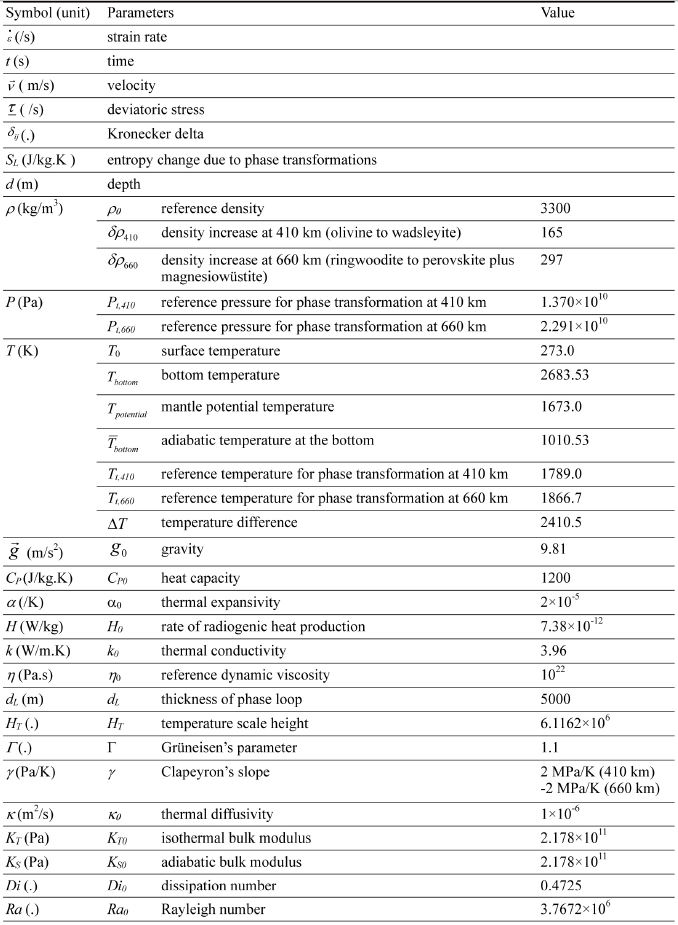
The governing equations used in this study are based on the incompressible Boussinessq approximation, described in previous studies (Ita and King, 1994; Lee and King, 2011). Thus, we briefly describe the governing equations for the mantle convection with phase transformations using the model symbols and parameters in Table 1, described below,

Model symbols and parameters.
| - continuity equation (1) |
| - momentum equation (2) |
| - energy equation (3) |
where the mantle density is expressed by the reference density plus density perturbations, described as,
| - mantle density (4) |
| - density perturbation (5) |
| - progress function (6) |
| - mantle temperature (7) |
| - mantle pressure (8) |
where ρ0 is the reference density, ρ' is the density perturbation, a function of the thermal expansion (T') and phase transformation (∏). π410and π660 are the progress functions (Richter, 1973) corresponding to the two major phase transformations in the mantle; ol to wd (a depth of 410 km) and rw to pv+ mw (a depth of 660 km), respectively (Ito and Takahashi, 1989; Fei et al., 2004; Akaogi et al., 2007).
The entropy changes due to phase transformations can be approximated by using the Clausius-Clapeyron and volume-density relations (Ita and King, 1994), described below;
| - entropy change (9) |
By applying the non-dimensionalization and keeping the original descriptions for a convenience, the governing equations are reduced as,
| - continuity equation (10) |
| - momentum equation (11) |
| - energy equation (12) |
In order to solve the governing equations with the model parameters, we used the finite element code, ConMan (King et al., 1990) used in Lee and King (2011). The penalty method (Hughes, 1987) is used for solving the continuity and momentum equations. The Streamline Upwind Petrov-Gelerkin (Hughes and Brooks, 1979) is used for solving the energy equation using the second-order predictor and corrector time-stepping scheme.
2.2 Rheology
The rheology used in this study is described in Lee and King (2011) and the plastic lithospheric deformation in Tackely (2000) is used,
| - yielding strength (13) |
where z' σbrittle and σductile correspond to brittle and ductile strength, respectively; the brittle strength is 0 at the top and 1 at the bottom.
Viscous mantle flow (Hirth and Kohlstedt, 2003; Karato and Wu, 1993) is used;
| - mantle viscosity (14) |
| - diffusion creep (15) |
| - dislocation creep (16) |
The effective viscosity governing the deformation of lithosphere and mantle is calculated;
| - effective viscosity (17) |
where the detailed explanations and values for the parameters are described in Table 2.
Model symbols and parameters for rheology.
2.3 Model setup
The model geometry used in this study is the same used in Lee and King (2011). The domain of the numerical experiments consists of 164 by 578 four-node quadrilateral elements for 2,890 by 11,560 km (1 by 4) (Figure 1). Because the phase transformations occur through thin phase loops (5 km), we used rectangular elements spanning a width-height range of 20 by 5 km from 380 to 440 km and from 620 to 690 km. Otherwise, 20 by 20 km elements are used throughout the remainder of the domain (Figure 1b). The megathrust where the converging plate sinks is implemented as a diagonal weak zone (27 degree) at the top-center of the model domain (5,780 km).

Model domain, grid distribution, viscosity profiles and initial temperature profile. a) Schematic diagram of the model domain used in this study. The dashed lines correspond to depths of 410, 660 and 2690 km. The reflected condition is used for the experiments. b) Grid distribution in the model domain. The two gray zones consist of 20 by 5 km elements whereas the other zone consists of 20 by 20 km elements. c) Viscosity profiles corresponding to 4-, 16- and 64-fold viscosity increases with a weak core-mantle boundary and the reference strain rate of 10-15/s. The other viscosity profiles for the larger viscosity increases are omitted for a clarity. For the upper mantle, activation volumes of the diffusion and dislocation creeps linearly decrease with depth by 30% at the 660 km discontinuity (Table 2). For the lower mantle, activation volume is kept constant with depth. Viscosity increases across the 660 km discontinuity are implemented by increasing the grain sizes, described in Table 2. d) Initial total temperature profile implemented in the model consisting of net mantle adiabat plus mantle potential temperature.
Constant temperatures are applied to the surface and bottom boundaries, and the side-walls are insulated boundaries. To avoid the symmetric subduction, the right side plate (continental plate) is fixed (no-slip) and free-slip boundary conditions are applied to all the remainder. The oceanic crust is forcefully subducted for 4 Myr with a convergence rate of 5 cm/a in order to accumulate initial buoyancy for the dynamic subduction. The whole mantle temperature is implemented by adding the half-space cooling model with a mantle potential temperature of 1,673 K and the net mantle adiabat. A uniform thickness of plates corresponding to 120 Ma is used for the continental plate (Stein and Stein, 1992). The oceanic plate is prescribed using the half-space cooling model for a constant spreading rate of 5 cm/a. The initial viscosity and temperature profiles are described in Figure 1c and d.
3. Results
Because the effect of viscosity increases across the discontinuity at a depth of 660 km on the buckling behavior of the subducting slab is described in Lee and King (2011), we primarily focus the effect of phase transformations on buckling behavior of the subducting slab.
3.1 Effect of earth-like phase transformations on buckling behavior of the subducting slab
Because Clapeyron’s slopes and density increases of the phase transformations are not well constrained (Dziewonski and Anderson, 1981; Bina and Wood, 1987; Duffy, 2005; Frost, 2008 and references therein), we used nominal Clapeyron’s slopes of 2 and -2 MPa/K, and density increases of 5 and 9% for the phase transformations from ol to wd and from rw to pv + mw, respectively. Including the phase transformations, we perform a series of experiments using the maximum slab viscosities of 1024 and 1026 Pa·s, corresponding to weak and strong slabs, respectively. For each set of the experiments, we vary the viscosity increase across the 660 km discontinuity as 4, 16, 32, 48, 64, 80, 96, 112 and 128 folds, used in Lee and King (2011).
First, we evaluate the experiments using the maximum slab viscosity of 1024 Pa·s. All the experiments except for the experiment using a 4-fold viscosity increase develop extensive buckling behavior of the subducting slab, though buckling in the experiment using a 16-fold viscosity increase is weaker than those in the other experiments; phase transformations result in a positive effect on the development of slab buckling (Table 3). Figure 2 shows a comparison of the experiments using an 80-fold viscosity increase with or without phase transformations. The phase transformation from ol to wd (a depth of 410 km) accelerates slab sinking and results in increased convergence rate compared with the experiments without the phase transformation. However, the phase transformation from rw to pv + mw retards slab sinking into the lower mantle and the subducting slab tends to be accumulated in the transformation (transition) zone (Figure 2a vs. 2b). Since the core of the retarded slab is more isolated from the hot adjacent mantle, cold core of the sinking slab in the lower mantle can be preserved for a longer time (Figure 2c vs. 2d).

Slab trajectories, slab temperatures, convergence rate and buckling amplitude of the experiments using an 80-fold viscosity increase with or without phase transformations. a) Slab trajectories at 58.27, 111.24 and 158.91 Myr since the experiment run without phase transformations. The slab trajectories are depicted using tracers implemented in the converging oceanic plate to the trench. The inverted triangle indicates the trench. Two dashed lines correspond to the depths of 410 and 660 km where phase transformations occur. b) Same with a except for including phase transformations. c) Slab temperatures at 119.18 Myr since the experiment run without phase transformations. Temperature is depicted every 200˚C. d) Same with c except for including phase transformations. e) Convergence rate of the incoming oceanic plate measured at the trench in the experiments with or without phase transformations. f) Buckling amplitude of the subducting slab in the experiments with or without phase transformations. The buckling amplitude is estimated by measuring the location of the implemented tracers of the subducting slab passing at a depth of 660 km.
Buckling parameters for the experiments using the maximum slab viscosity of 1024 Pa․s and 410 and 660 km phase transformations.
Using the buckling parameters, buckling analysis is conducted using the scaling laws (Ribe et al., 2007). The scaling laws for the amplitude (δ) and period (φ) of the buckling slab can be shown by;
| - amplitude of slab buckling (18) |
| - period of slab buckling (19) |
where H0 is the effective fall height indicating the distance between the earth’s surface and 660 km discontinuity, d is the slab thickness and U0 is the mean convergence rate. Buckling analyses show that the scaling laws generally predict the buckling amplitude and period of the subducting slab with small relative errors (mostly < 20% except for the first and last buckling of the subducting slab). Despite the heterogeneous slab composition due to the phase transformations is not considered the scaling laws predict the buckling behavior of the subducting slab.
Next, we evaluate the effect of the phase transformations using the maximum slab viscosity of 1026 Pa·s. As observed in Lee and King (2011), strong slab weakens buckling behavior of the subducting slab, expressed as small buckling amplitudes and cycles (Figure 3a vs. 3c) and increases buck ling periods (Figure 3b vs. 3d). Except for these observations, the effect of viscosity increase across the 660 km discontinuity on the buckling behavior is very similar to the experiments using the maximum viscosity of 1024 Pa·s (weak slab). The buckling analyses show that the experimentsusing strong slab results in somewhat larger relative errors in buckling amplitudes and periods compared with the experiments using weak slab but, the errors are not considerably large (Table 4). Both sets of experiments varying the maximum slab viscosity show that the scaling laws predict the buckling behavior of the subducting slab even the phase transformations are included.

Buckling amplitudes and periods in the experiments with or without phase transformations. a and b) Estimated buckling amplitude and buckling period of the experiments using the maximum viscosity of 1024 Pa․s and both phase transformations occurred at depths of 410 and 660 km. Viscosity increases correspond to the viscosity increases across the discontinuity at a depth of 660 km. Cycles correspond to the measured buckling amplitudes and periods described in Table 4. c and d) Same with a and b except for the experiments using the maximum viscosity of 1026 Pa․s. e and h) Buckling amplitudes and periods in the experiments using a 32-fold viscosity increase and the phase transformation occurring at a depth of 410 km. The Clapeyron’s slope varies as 1, 2 and 3 MPa/K. f and i) Same with f and i except for in the experiment using a 64-fold viscosity increase. g and j) Same with f and i except for in the experiment using a 96-fold viscosity increase. k and n) Buckling amplitudes and periods in the experiments using a 32-fold viscosity increase and the phase transformation occurring at a depth of 660 km. The Clapeyron’s slope varies -1, -2 and -3 MPa/K. l and o) Same with k and n except for in the experiments using a 64-fold viscosity increase. m and p) Same with k and n except for in the experiments using a 96-fold viscosity increase.
Buckling parameters for the experiments using the maximum slab viscosity of 1026 Pa․s and 410 and 660 km phase transformations.
3.2 Effect of each phase transformation on buckling behavior of the subducting slab
Along with the experiments using both phase transformations, we evaluate each contribution of the phase transformations to the buckling behavior of the subducting slab by switching on and off individual phase transformations from ol to wd and from rw to pv + mw. First, we vary the Clapeyron’s slope of the phase transformation from ol to wd as 1, 2 and 3 MPa/K without the phase transformation from rw to pv + mw. Regarding the viscosity increases across the discontinuity at a depth of 660 km, 32-, 64-, and 96-fold viscosity increases are selected and the maximum slab viscosity is fixed as 1024 Pa·s to avoid many unnecessary additional experiments. Other parameters are the same with the experiments described above.
Except for the experiment using the Clapeyron’s slope of 1 MPa/K and 32-fold viscosity increase, all the experiments develop several cycles of slab buckling and the averaged convergence rate of each buckling cycle except for the last cycle generally increases with time in all the experiments. As observed in the experiments using both phase transformations, the scaling laws predict the buckling behavior of the subducting slab with small errors (Figure 3e-j and Table 5). It clearly indicates that increased slab pull due to the endothermic phase transformation accelerates slab sinking in the upper mantle and the subducting slab reaches the 660 km discontinuity in a shorter time. The averaged convergence rate per each cycle of slab buckling increases with the Clapeyron’s slope, indicating a positive effect of the endothermic phase transformation on slab pull (Figure 4a-c). The endothermic phase transformation reduces the required viscosity increase for slab buckling across the 660 km discontinuity because the accelerated slab is not accommodated by slab sinking in the lower mantle but laterally deformed.

Slab trajectories in the experiments by switching on or off the phase transformations from olivine (ol) to wadsleyite (wd) and from ringwoodite (rw) to perovskite (pv) plus magnesiowüstite (mw). The snapshots of the slab trajectories are taken on 56.9, 109.9 and 162.9 Myr since the experiment run. The dashed lines correspond to depths of 410 and 660 km where the two phase transformations occur. a, b and c) Slab trajectories corresponding to the Clapeyron’s slopes for the phase transformation from olivine to wadsleyite at a depth of 410 km as 1, 2 and 3 MPa/K. The Clapeyron’s slope of 0 MPa/K indicates no phase transformation at a depth of 660 km. d) Slab trajectories in the experiments without phase transformations. e) Slab trajectories in the experiments with the two phase transformations of which Clapeyron’s slopes of 2 and -2 MPa/K, respectively. f, g and h) Slab trajectories corresponding to the Clapeyron’s slopes for the phase transformation from ringwoodite to perovskite plus magnesiowüstite as -1, -2 and -3 MPa/K. 0 MPa/K indicates no phase transformation at a depth of 410 km.
Next, we vary the Clapeyron’s slope of the phase transformation from rw to pv + mw as -1, -2, and -3 MPa/K without the phase transformation from ol to wd. As expected, the phase transformation significantly retards slab sinking and results in stacked slab on the 660 km discontinuity, especially, in the experiments using the Clapeyron’s slopes of -2 and -3 MPa/K (Figure 4f-h). The stacked slab is attributed to sluggish slab penetration to the 660 km discontinuity, slab buckling mostly occurs in the transformation zone of the upper mantle, different than the slab buckling in the shallow lower mantle in the experiments above. The stacked slab on the discontinuity abruptly falls into the lower mantle due to the accumulated negative buoyancy of the slab itself (162.8 Myr in Figure 4f and 4g). Since the slab avalanche, the subducting slab descends with little slab buckling because the extensional (pulling) stress guide of the descending stacked slab in the lower mantle prevents buckling in the transformation zone. In the experiment using the Clapeyron’s slope of -3 MPa/K, the subducting slab is significantly accumulated on the 660 km discontinuity and sinking in the lower mantle is considerably frustrated. Because the buckling amplitude is estimated by using the implemented tracers in the slab path, the buckling amplitude in the accumulated slab cannot be precisely measured; the scaling laws only predict very early cycles of the buckling behavior of the subducting slab (Figures 3m, 3p, 4h and Table 6).
From the experiments above, we find that the phase transformation from olto wd develops fairly regular buckling amplitude of the subducting slab by the subduction termination due to slab detachment (Figure 4a-c and Table 5). However, the phase transformation from rw to pv + mw significantly retards slab sinking in the shallow lower mantle. The accumulated negative buoyancy results in abrupt slab sinking in the deep lower mantle similar to the slab avalanche and buckling behavior of the subducting slab is significantly weakened, which is not observed in the experiments using the phase transformation from ol to wd. Since the effect of two phase transformations on the buckling behavior of the subducting slab is cancelled out each other, the experiments using both phase transformations can develop similar style of slab buckling observed in the experiments without phase transformations (Figure 4d vs. 4e).
Buckling parameters for the experiments using the maximum slab viscosity of 1024 Pa․s and 410 km phase transformation.
Buckling parameters for the experiments using the maximum slab viscosity of 1024 Pa․s and 660 km phase transformation only.
4. Discussion
Lee and King (2011) shows that the buckling behavior of the subducting slab is consistent with the scaling laws for the buckling behavior of the descending fluid and explains the time-evolving convergence rate of the oceanic plate, randomly distributed slab dip in the upper mantle and time-evolving back-arc stress environments in the subduction zones. Further studies to investigate the effect of phase transformations on buckling behavior of the subducting slab are conducted here. Results show that phase transformation plays an important role in the buckling behavior of the subducting slab. The endothermic phase transformation from ol to wd at a depth of 410 km accelerates the subducting slab, and lateral slab deformation (buckling) in the shallow lower mantle accommodates the fast subducting slab, observed in a previous study (Behounková and Cízková, 2008). Thus, smaller viscosity increase across the discontinuity at a depth of 660 km results in slab buckling compared with that in the experiments without phase transformations. The exothermic phase transformation from rw to pv+ mw at a depth of 660 km retards the slab penetration to the lower mantle; the subducting slab tends to stack on the 660 km discontinuity rather than sinking into the lower mantle with longer buckling cycles than that of the experiments without phase transformations. The faster convergence rate and shorter buckling period of the experiments using the both phase transformations are attributed to both acceleration (downward push) of slab sinking by the phase transformation from ol to wd and retardation (upward resistance) of slab sinking by the phase transformation from rw to pv+ mw. Despite the existence of phase transformations, the scaling laws predict buckling behavior of the subducting slab with relatively small errors (< 20%). Thus, the scaling laws successfully predicts bucking behavior of the subducting slab influenced by phase transformations.
The results above indicate that the scaling laws can be successfully applied to the buckling behavior in the earth-like mantle. The subduction zones in Java-Sunda, Central America and South America develop apparent slab thickening in the shallow lower mantle, consistent with the buckling analyses using the scaling laws (Ren et al., 2007; Ribe et al., 2007; Schellart et al., 2007). Other subduction zones relevant to our model calculations may be the subduction zones in Northeast Japan and Izu. Seismic tomography images show that apparently thickened slab in the transformation zone so called ‘megalith’ (Ringwood and Irifune, 1988; Gu et al., 2012), implying slab buckling in the transformation zone. The compressional back-arc stress environment, shallow slab dip and increasing convergence rate of the incoming Pacific plate to the subduction zones (Sdrolias and Müller, 2006) are plausible observations indicating that the buckling behavior of the subducting slab occurs even in the transformation zone. It is well consistent with our model calculations that the phase transformation from ol to wd significantly contributes to slab buckling in the transformation zone and periodic evolution of the plate motion. In addition, seismic tomography images indicating the thickened subducted Farallon plate in the transformation zone (Schmid et al., 2002) suggest that buckling behavior of the subducting slab occurs even if the subducting slab accumulates in the transformation zone without the slab penetration to the lower mantle.
In this study, except for the viscosity governed by plastic rheology in shallow depth, the viscosity of the subducting slab is controlled by temperature, density and strain rate (upper mantle) expressed as the Arrhenius type viscosity equation. However, water, pre-developed faults/cracks and grain size reduction in the subducting slab, not considered in the viscosity equation, may significantly reduce the effective slab strength (Ranalli, 1991; Riedel and Karato, 1997; Hirth and Kohlstedt, 2003). For example, the reduced grain size of the subducting slab by the phase transformation from ol to wd in the upper mantle (Riedel and Karato, 1997) results in weaker slab strength in the lower mantle than our calculations and may result in more buckling cycles and shorter period (wavelength) of slab buckling. In addition, laboratory experiments show that thermal expansivity and conductivity of the mantle are pressure- and temperature-dependent (Hofmeister, 1999; Liu and Li, 2006). If the thermal expansivity and conductivity of the subducting slab decreases and increases with depth, respectively, the reduced negative slab buoyancy retards its descending to the lower mantle (Ita and King, 1998); slab buckling may be more prevalent than our model calculations.
The relationship between periodic buckling behavior of the subducting slab and resultant periodic convergence rate of the incoming plate has a potential implication for subduction zone tectonics. Lee and King (2011) show that the periodic convergence rate of the incoming oceanic plate, an expression of the slab buckling, is correlated to the alternating compressional and extensional back-arc stress environment in Cenozoic South America. Another example implying the relationship between periodic buckling behavior of the subducting slab and alternating compressional and extensional back-arc stress environment is the Cretaceous Gyeongsang basin in Southeast Korean Peninsula. Previous studies suggested that the Gyeongsang basin experienced several alternating back-arc extensions and compressions due to changes in the subduction direction of the Izanagi plate along the NE-SW extending trench located in southeastern region of the basin (Sagong et al., 2005; Ryu et al., 2006). Another recent study shows that the roll-back of the Izanagi plate since 130 Ma resulted in eastward trend sedimentations in the Gyeongsang basin (Chough and Sohn, 2010). However, a recent plate reconstruction model (Sdrolias and Müller, 2006; Gurnis et al., 2012) shows that the Izanagi plate experienced changes in convergence direction, periodic evolution of the convergence rate and decreasing age of the subducting slab (Figure 5a-d, e and f). The total velocity constrained from the plate reconstruction model implies buckling behavior of the subducting slab; the Izanagi plate may result in the three alternating back-arc compressions and extensions in the Gyeongsang basin. As shown in Lee and King (2011), the age of the subducting slab does not significantly affect the buckling behavior of the subducting slab. Thus, the decreasing slab age may not significantly affect the tectonic evolution. Although the effect of changes in convergence direction on the buckling behavior has not been evaluated, it implies that the time-evolving motion of the oceanic plate can be used for understanding tectonic evolution of ancient subduction zones including the Gyeongsang basin.

Plate reconstruction model of the Cretaceous East Asia from 140 Ma to 60 Ma. a, b, c and d) Snapshots of the plate reconstruction on 130, 110, 80 and 70 Ma are prepared using the GPlate software (Boyden et al., 2011; Gurnis et al., 2012). The Gyeoungsang basin is located in Southeast Korean Peninsula, depicted as the white star. The black arrows indicate the convergence direction of the Izanagi (IZ) and Pacific (PA) plates toward the Eurasian (EU) plate. e) Evaluated total velocity (rate) of the converging Izanagi plate toward the Eurasian plate. The black boxes are plate ages picked up every 5 Myr from the plate reconstruction model and the convergence rate is approximated using piecewise polynomials. Subduction direction is calculated using the averaged plate motion every 10 Myr. The alphabets of the blue es and red cs correspond to extension and compression, respectively. f) Slab age constrained by the plate reconstruction model. The black pyramids correspond to the picked slab ages every 5 Myr from the plate reconstruction model and the slab age is approximated using piecewise polynomials.
5. Conclusion
In this study, we examine the effect of phase transformations on the buckling behavior of the subducting slab and suggest its tectonic implication. The phase transformation from olivine to wadsleyite at a depth of 410 km plays an important role in the development of slab buckling; increased slab pull due to the endothermic phase transformation accelerates slab sinking in the upper mantle and the subducting slab reaches the 660 km discontinuity in a shorter time than that of the experiments without the phase transformation. The averaged convergence rate per each cycle of slab buckling increases with the Clapeyron’s slope, indicating a positive effect of the endothermic phase transformation on slab pull. The phase transformation also reduces the viscosity increase required for the onset of periodic slab buckling compared with the experiments without phase transformations. However, the phase transformation from ringwoodite to perovskite plus magnesiowüstite only contributes to a minor role in the development of slab buckling; the phase transformation retards slab sinking into the lower mantle and the subducting slab tends to be accumulated in the transformation zone above the 660 km discontinuity. This study shows that the phase transformation from olivine to wadsleyite, neglected in many previous studies, significantly contributes to periodic plate motion and buckling behavior of the stagnant slab in the transformation zone. Buckling analyses show that the scaling laws generally predict the buckling amplitude and period of the subducting slab with small relative errors even if the phase transformations are considered.
The model calculations including the phase transformations show that buckling of the subducting slab is a universal process occurring in the mantle. In the subduction zones in Java-Sunda, Central America and South America as well as Northeast Japan and Izu, apparent slab thickening in the shallow lower mantle is consistent with the buckling behavior of the subducting slab in our model calculations. Although further studies should be required, the periodic compressions and extensions to the Cretaceous Gyeongsang basin could be related to the buckling behavior of the subducting Izanagi plate.
Acknowledgments
이 논문을 심사해 주신 두 분의 심사위원님과 편집위원장님에게 감사 드립니다. 이 연구는 한국연구재단(2016R1D1A1B03930906)과 기상청 기상·지진 See-At기술개발연구(KMI 2017-9090)의 지원으로 수행되었습니다.
References
- Akaogi, M., Takayama, H., Kojitani, H., Kawaji, H., and Atake, T., (2007), Low-temperature heat capacities, entropies and enthalpies of Mg2SiO4 ploymorphs, and α-β-γ and post-spinel phase relations at high pressure, Physics and Chemistry of Minerals, 34, p169-183.
- Behounková, M., and Cízková, H., (2008), Long-wavelength character of subducted slabs in the lower mantle, Earth and Planetary Science Letters, 275, p43-53.
-
Billen, M.I., and Hirth, G., (2007), Rheologic controls on slab dynamics, Geochemistry Geophysics Geosystems, 8(Q08012).
[https://doi.org/10.1029/2007gc001597]

-
Bina, C., and Wood, B., (1987), Olivine-spinel transitions: Experimental and thermodynamic constraints and implications for the nature of the 400-km seismic discontinuity, Journal of Geophysical Research, 92, p4853-4866.
[https://doi.org/10.1029/jb092ib06p04853]
-
Chough, S.K., and Sohn, Y.K., (2010), Tectonic and sedimentary evolution of a Cretaceous continental arc-backarc system in the Korean peninsula: New view, Earth-Science Reviews, 101, p225-249.
[https://doi.org/10.1016/j.earscirev.2010.05.004]
-
Christensen, U.R., (1996), The influence of trench migration on slab penetration into the lower mantle, Earth and Planetary Science Letters, 140, p27-39.
[https://doi.org/10.1016/0012-821x(96)00023-4]
-
Christensen, U.R., (1997), Influence of chemical buoyancy on the dynamics of slabs in the transition zone, Journal of Geophysical Research-Solid Earth, 102, p22435-22443.
[https://doi.org/10.1029/97jb01342]
-
Christensen, U.R., and Yuen, D.A., (1985), Layered convection induced by phase-transitions, Journal of Geophysical Research, 90, p291-300.
[https://doi.org/10.1029/jb090ib12p10291]
-
Cserepes, L., Yuen, D.A., and Schroeder, B.A., (2000), Effect of the mid-mantle viscosity and phase-transition structure on 3D mantle convection, Physics of the Earth and Planetary Interiors, 118, p135-148.
[https://doi.org/10.1016/s0031-9201(99)00140-5]
-
Duffy, T.S., (2005), Synchrotron facilities and the study of the Earth's deep interior, Reports on Progress in Physics, 68, p1811-1859.
[https://doi.org/10.1088/0034-4885/68/8/r03]
-
Dziewonski, A.M., and Anderson, D.L., (1981), Preliminary reference earth model, Physics of the Earth and Planetary Interiors, 25, p297-356.
[https://doi.org/10.1016/0031-9201(81)90046-7]
- Elliott, T., (2003), Tracers of the slab, In: Eiler J (ed.) Inside the Subduction Factory, Washington, DC: American Geophysical Union, 138, p23-43.
-
Fei, Y., Van Orman, J., Li, J., van Westrenen, W., Sanloup, C., Minarik, W., Hirose, K., Komabayashi, T., Walter, M., and Funakoshi, K., (2004), Experimentally determined postspinel transformation boundary in Mg2SiO4 using MgO as an internal pressure standard and its geophysical implications, Journal of Geophysical Research, 109.
[https://doi.org/10.1029/2003jb002562]
-
Frost, D.J., (2008), The Upper Mantle and Transition Zone, Elements, 4, p171-176.
[https://doi.org/10.2113/gselements.4.3.171]
-
Fukao, Y., Widiyantoro, S., and Obayashi, M., (2001), Stagnant slabs in the upper and lower mantle transition region, Review of Geophysics, 39, p291-323.
[https://doi.org/10.1029/1999rg000068]
-
Gaherty, J.B., and Hager, B.H., (1994), Compositional vs thermal buoyancy and the evolution of subducted lithosphere, Geophysical Research Letters, 21, p141-144.
[https://doi.org/10.1029/93gl03466]
-
Griffiths, R.W., and Turner, J.S., (1988), Folding of Viscous Plumes Impinging On A Density Or Viscosity Interface, Geophysical Journal, 95, p397-419.
[https://doi.org/10.1111/j.1365-246x.1988.tb00477.x]
- Gu, Y.J., Okeler, A., and Schultz, R., (2012), Tracking slabs beneath northwestern Pacific subduction zones, Earth and Planetary Science Letters, p331–332-269-280.
-
Guillou-Frottier, L., Buttles, J., and Olson, P., (1995), Laboratory experiments on the structure of subducted lithosphere, Earth and Planetary Science Letters, 133, p19-34.
[https://doi.org/10.1016/0012-821x(95)00045-e]
-
Gurnis, M., and Hager, B.H., (1988), Controls of the structure of subducted slabs, Nature, 335, p317-321.
[https://doi.org/10.1038/335317a0]
-
Gurnis, M., Turner, M., Zahirovic, S., DiCaprio, L., Spasojevic, S., Müller, R.D., Boyden, J., Seton, M., Manea, V.C., and Bower, D.J., (2012), Plate tectonic reconstructions with continuously closing plates, Computers & Geosciences, 38, p35-42.
[https://doi.org/10.1016/j.cageo.2011.04.014]
- Hirth, G., and Kohlstedt, D., (2003), Rheology of the Upper Mantle and the Mantle Wedge: A View from the Experimentalists, in Inside the Subduction Factory, Geophysical Monograph, 138, p83-105.
-
Hofmeister, A.M., (1999), Mantle Values of Thermal Conductivity and the Geotherm from Phonon Lifetimes, Science, 283, p1699-1706.
[https://doi.org/10.1126/science.283.5408.1699]
- Hughes, T., (1987), The Finite Element Method: Linear Static and Dynamics Finite Element Analysis, Couricr Corporation.
- Hughes, T.J.R., and Brooks, A., (1979), 'A multidimensional upwind scheme with no crosswind diffusion', in T. J. R. Hughes, ed, Finite element methods for convection dominated flows, AMD 34, 19-35, Presented at the Winter Annual Meeting of the ASME, Amer, Amer. Soc. Mech. Engrs. (ASME), New York.
-
Ita, J., and King, S.D., (1994), Sensitivity of convection with an endothermic phase change to the form of governing equations, initial conditions, boundary conditions, and equation of state, Journal of Geophysical Research-Solid Earth, 99, p15919-15938.
[https://doi.org/10.1029/94jb00852]
-
Ita, J., and King, S.D., (1998), The influence of thermodynamic formulation on simulations of subduction zone geometry and history, Geophysical Research Letters, 25, p1463-1466.
[https://doi.org/10.1029/98gl51033]
-
Ito, E., and Takahashi, E., (1989), Postspinel Transformations in the System Mg2SiO4-FeSiO4 and Some Geophysical Implications, Journal of Geophysical Research, 94, p10637-10646.
[https://doi.org/10.1029/jb094ib08p10637]
- Karason, H., and van der Hilst, R.D., (2001), Tomographic imaging of the lowermost mantle with differential times of refracted and diffracted core phases (PKP, P-diff), Journal of Geophysical Research, 106, p6569-6587.
-
Karato, S.-I., and Wu, P., (1993), Rheology of the upper mantle: a synthesis, Science, 260, p771-778.
[https://doi.org/10.1126/science.260.5109.771]
-
King, S.D., (2002), Geoid and topography over subduction zones: The effect of phase transformations, Journal of Geophysical Research, 107.
[https://doi.org/10.1029/2000jb000141]
- King, S.D., (2007), Mantle Downwellings and the Fate of Subducting Slabs: Constraints from Seismology, Geoid Topography, Geochemistry, and Petrology, in: Gerald, S. (Ed.), Treatise on Geophysics, Elsevier, Amsterdam, p325-370.
-
King, S.D., and Ita, J., (1995), Effect of slab rheology on mass-transport across a phase-transition boundary, Journal of Geophysical Research, 100, p20211-20222.
[https://doi.org/10.1029/95jb01964]
-
King, S.D., Raefsky, A., Hager, B.H., (1990), Conman: vectorizing a finite element code for incompressible two-dimensional convection in the Earth's mantle, Physics of the Earth and Planetary Interiors, 59, p195-207.
[https://doi.org/10.1016/0031-9201(90)90225-m]
-
Lee, C., and King, S.D., (2011), Dynamic buckling of subducting slabs reconciles geological and geophysical observations, Earth and Planetary Science Letters, 312, p360-370.
[https://doi.org/10.1016/j.epsl.2011.10.033]
-
Liu, W., and Li, B., (2006), Thermal equation of state of (Mg0.9Fe0.1)2SiO4 olivine, Physics of the Earth and Planetary Interiors, 157, p188-195.
[https://doi.org/10.1016/j.pepi.2006.04.003]
- Ranalli, G., (1991), The microphysical approach to mantle rheology, In: Sabadini, R., Lambeck, K., Boschi, E. (Eds.), Glacial Isostacy, Sea-Level and Mantle Rheology, p343-378.
-
Ren, Y., Stutzmann, E., van der Hilst, R.D., and Besse, J., (2007), Understanding seismic heterogeneities in the lower mantle beneath the Americas from seismic tomography and plate tectonic history, Journal of Geophysical Research, 112(B01302).
[https://doi.org/10.1029/2005jb004154]
-
Ribe, N.M., (2003), Periodic folding of viscous sheets, Physical Review E, 68(036305).
[https://doi.org/10.1103/physreve.68.036305]
-
Ribe, N.M., Stutzmann, E., Ren, Y., and van der Hilst, R., (2007), Buckling instabilities of subducted lithosphere beneath the transition zone, Earth and Planetary Science Letters, 254, p173-179.
[https://doi.org/10.1016/j.epsl.2006.11.028]
-
Richter, F.M., (1973), Dynamical models for sea floor spreading, Review of Geophysics, 11, p223-287.
[https://doi.org/10.1029/rg011i002p00223]
-
Riedel, M.R., and Karato, S.-I., (1997), Grain-size evolution in subducted oceanic lithosphere associated with the olivine-spinel transformation and its effects on rheology, Earth and Planetary Science Letters, 148, p27-43.
[https://doi.org/10.1016/s0012-821x(97)00016-2]
-
Ringwood, A.E., and Irifune, T., (1988), Nature of the 650-km seismic discontinuity: implications for mantle dynamics and differentiation, Nature, 331, p131-136.
[https://doi.org/10.1038/331131a0]
- Ryu, I.-C., Choi, S.G., and Wee, S.M., (2006), An Inquiry into the Formation and Deformation of the Cretaceous Gyeongsang (Kyongsang) Basin, Southeastern Korea, Economic and Environmental Geology, 39, p129-149.
-
Sagong, H., Kwon, S.-T., and Ree, J.-H., (2005), Mesozoic episodic magmatism in South Korea and its tectonic implication, Tectonics, 24(TC5002).
[https://doi.org/10.1029/2004tc001720]
-
Schellart, W.P., Freeman, J., Stegman, D.R., Moresi, L., and May, D., (2007), Evolution and diversity of subduction zones controlled by slab width, Nature, 446, p308-311.
[https://doi.org/10.1038/nature05615]
-
Schmid, C., Goes, S., van der Lee, S., and Giardini, D., (2002), Fate of the Cenozoic Farallon slab from a comparison of kinematic thermal modeling with tomographic images, Earth and Planetary Science Letters, 204, p17-32.
[https://doi.org/10.1016/s0012-821x(02)00985-8]
-
Sdrolias, M., and Müller, R.D., (2006), Controls on back-arc basin formation, Geochemistry Geophysics Geosystems, 7.
[https://doi.org/10.1029/2005gc001090]
-
Stein, C.A., and Stein, S., (1992), A model for the global variation in oceanic depth and heat flow with lithospheric age, Nature, 359, p123-129.
[https://doi.org/10.1038/359123a0]
- Stern, R.J., (2002), Subduction zones, Review of Geophysics, 40(1012).
-
Tackley, P.J., (1995), Mantle dynamics - influence of the transition zone, Reviews of Geophysics, 33, p275-282.
[https://doi.org/10.1029/95rg00291]
-
Tackley, P.J., (2000), Self-consistent generation of tectonic plates in time-dependent, three-dimensional mantle convection simulations, Geochemistry, Geophysics, Geosystems, 1.
[https://doi.org/10.1029/2000gc000036]
- Taylor, G.I., (1968), Instability of jets, threads, and sheets of viscous fluid, Proc. Twelfth Int. Cong. Appl. Mech, Springer Verlag, Berlin.
-
Tome, M.F., and McKee, S., (1999), Numerical simulation of viscous flow: Buckling of planar jets, International Journal for Numerical Methods in Fluids, 29, p705-718.
[https://doi.org/10.1002/(sici)1097-0363(19990330)29:6<705::aid-fld809>3.3.co;2-3]
-
van Keken, P.E., (2003), The structure and dynamics of the mantle wedge, Earth and Planetary Science Letters, 215, p323-338.
[https://doi.org/10.1016/s0012-821x(03)00460-6]